Rebecca D Wooten*
Department of Mathematics and Statistics, University of South Florida, USA
Received date: 21/08/2016; Accepted date: 24/08/2016; Published date: 27/08/2016
Visit for more related articles at Research & Reviews: Journal of Statistics and Mathematical Sciences
Implicit regression, Bivariate, Non-linear regression, Coefficient of variation, Model quality.
Non-Response analysis uses ordinary least squares and maximum likelihood estimates to fit co-dependent variables in an implicit form including conic sections such as circles, ellipse, hyperbolas, and spheres, among other higher dimensional surfaces.
Conic sections in 2-dimensions are relationships between two measures that take the form

This form includes lines, circles, ellipse, parabolas and hyperbolas [1,2].
Consider an example in a conical relationship:

Simulation of an Ellipse
To simulate an ellipse, let time ‘t’, be taken in random intervals over one unit of measurement,

To simulate an ellipse, consider the transformed space (u, v) such that in the first direction, the measure u moves linearly over time, either increasing or decreasing at a rate of 3 units per unit measure of time,  and in the second direction, the measure
  moves along one of two curves,
  Further transformation of the (u, v) space to the (x, y) space by rotating the resulting ellipse 45° counterclockwise, letting
  Random error exists in both variables:
  with a sample of size 100, (Figure 1).
Using standard regression on the full second-order model as given by,

Which only accounts for the central tendency and does not allow for the subject response to be conditional, (Figure 2a). The model can be improved slightly if we partition the data and fit points above this nearly linear equation (d =1) separately from those below the developed equation (d =1); that is,

This gives better point estimates then the single estimate, (Figure 2b).
Using non-response analysis on the full second-order interactive model,

And solving for  using the quadratic equation yields much better results, (Figure 3);

Where,  Note: if
  a line as shown outside of the ellipse in Figure 3a.
Compare this with the model full second-order model first for the data overall and using the partitioned data, (Figure 3b).
Non-response Analysis in Three-Dimensions
Non-response analysis can also model in multi-dimensional space and is only restricted by the tractability of the variable measures [3].
Non-response Analysis on Spheres
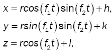
Consider more complex models such as data which lies in a spherical relationship that is observed over time. For example, consider the relationship between three variables, one considered to be the subject response, y, and the other two explanatory: x and z; and the true state of nature be outlined by,

For a sphere with fixed center (h, k, l) and fixed radius r.

where the time measured in random intervals for multiple cycles  and the three random error terms are normally distributed with a mean of zero and constant variance: that is τ, δ, and ε are

Just looking at the data, there is no apparent relationship other than the somewhat circular nature of the data (Figure 4).
Using regression on the full second-order interactive model,

This mainly accounts for the central tendency and does not allow for higher order terms and interaction with the subject response (Figure 5).
Using non-response analysis on the full second-order interactive model

And solving for y using the quadratic equation yields much better results, (Figure 6);

Where 
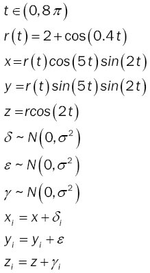
Consider the space of a sphere which is transforming over time as the radius oscillates between one and three [4,5].
Let time be randomly observed over a period of 8π, and three measures be such that  where r (t) is an unknown measure but is believe to change over time. For simulation purposes, the radius will be defined to be between one and three with a period of 5π. Furthermore, let each measured variable include random error that is normally distributed with expected value of zero and equal constant variance (Figures 7 and 8).

Modeling the spherical relationship given by

The coefficient of determination is approximately 0.7 which is a measure of the constant nature of the system and indicates that the constant that balances the system is highly variant with nearly a uniform distribution.
Using the developed model to estimate unity (the constant the balances the system), we see the ossilation is more clearly defined, (Figure 9) and from which the frequency of ossilation can be determined in addition to the range. In this simulation the range is two.
Furthermore, as each measured variable is expected to be zero, by considering the reduced model given by

Using the developed model  on average, we can estimate the mean radius using u, we have,
  In this simulation the radius was approximately two for each estimate of the radius.
In this review, analysis shows that non-response model allows for information about unmeasured variables to be detected and with proper modeling, estimated. Hence, non-response analysis can measure the constant nature of a single variable; measure the balancing constant in a stable system and estimate the subject response in an evolving system.