Modelling Monthly Inflation in the Philippines using Seasonal Autoregressive Integrated Moving Average (ARIMA)

Abstract

Inflation impacts the country's economy greatly. It is vital not only to the government, but also to the lifestyle of an average person. It plays a crucial role in decision-making done by households, firms, markets, and government. With the existing importance of inflation to a country, the role of forecasting becomes crucial. Better decision-making and reinforced preparations come with a good forecasting. Given that, this paper aims to model inflation rates in the Philippines in a Seasonal ARIMA (SARIMA) framework. The data used for modelling were monthly values from January 2015 to March 2020. Analysis reveals that inflation rates in the Philippines follow a seasonal ARIMA (0, 1, 0) (1, 1, 0) (12). The model has Mean Absolute Percentage Error (MAPE), Root Mean Square Error (RMSE) and Theil Inequality Coefficient value of 1.189417, 1.012582, and 0.089779, respectively. Therefore, the model is adequate since the values are close to zero. It is also shown to be accurate in forecasting inflation rates with an accuracy of 98.81058% for the 24-month forecast.

Keywords

Inflation; Prediction; modelling; SARIMA Subject classification codes: E31, C53, C55

Introduction

Inflation: effects and forecasting

In the years 1992-1995, it has been believed that inflation is dead. However, Yap said that this declaration is inaccurate as it has been based on flawed empirical evidence [1]. Based on Bangko Sentral ng Pilipinas report, inflation is still regarded as a threat to macroeconomic stability in the Philippines. Its effect ranges from the government to the households as Philippines remained to be one of the countries in Asia with high inflation rates. For the past years, policies made to stabilize the economy resulted in episodes of stagflation. This is brought by wrong decisions made by policymakers and economic managers.

According to Crowther, inflation is a state wherein the values of money fall as prices increase. It means your money could not buy today as much as you could buy yesterday. In a household setting, inflation has two different effects: asset inflation or income inflation [2]. If an asset is owned before price rise, it will have a larger value in the next years. An asset inflation affects the household positively. On the other hand, if household income does not keep pace with inflation, the buying power declines. Over time, income inflation increases your cost of living. Tolcha concluded that people perceived inflation as danger to their standards of living [3].

Inflation affects the businesses similarly. However, few excellent companies may view inflation as an opportunity. Inflation discourages productivity, leads to inefficient resource allocation, and may create future recessions. For some cases, it offers opportunities for differentiation. Companies must make informed and right decisions while assessing risks, understanding financial capacities and protect capital investments, in order to keep business from falling [4].

The degree of impact inflation will bring to the household depends on how the market responds. According to James, inflation is the persistent rise in prices caused by excess demand over supply. It can simply be expressed as “too many dollars, chasing too few goods.” The invisible hand, a concept that was first introduced by Adam Smith, describes the unintended social actions that benefit the market economy. However, with the existing phenomenon where both the firm and household affected, the government intervenes.

There are many methods that the government might use for to control inflation. One of the common methods is policymaking. The practice of forecasting inflation has generally been considered as an important input for the conduct of monetary policymaking. Central banks, specifically Bangko Sentral ng Pilipinas aims to achieve price stability need to be forward-looking in their decisions as well, which lies the importance of inflation forecasting.

The importance of inflation to economic growth highlights the need to model inflation. Whether in the household, firms, or to the policymakers, forecasting inflation plays a crucial role to achieve every entity’s goal for the betterment of the country’s economy. Better decision-making and reinforced preparations come with a good forecasting. An adequate forecasting model provides general indication of the likely environment in which forward-looking policy needs to be formulated.

Through decades, studies are done on finding models for inflation prediction. ARIMA time series models to predict Bangladesh’s inflation. The result showed that the best model to forecast for up to 5 years for the inflation in Bangladesh using 38-year data is ARIMA (1, 0, and 0). It is predicted to have an inflation rate of 4.40% in 2016, then rises to 4.65% in 2017 with a slightly increased rate in the next consecutive years [5].

Researchers in their studies on inflation forecasting garnered mixed results. It provides a comparative assessment of VAR and ARIMA models to forecast Austrian Harmonized Index of Consumer Prices inflation over the short term. The researchers found that VAR models are better than ARIMA models in terms of predictive accuracy. On the other hand, showed that the VAR models do not perform better than the ARIMA (2, 1, 2) models [6,7].

What makes inflation difficult to model is its seasonality. Seasonality is the presence of variation that occurs at regular time interval. The inflation in the Philippines is said to seasonal in a monthly basis. According to the Philippine Statistics Authority (PSA), the country's inflation rate rose from 6.4% in August to 6.7% in September 2018, the highest in over 9 years. It was also the 9th consecutive monthly inflation rate increase, which started in January 2018. On the other hand, the Philippines’ headline inflation decelerated further to 1.7 percent in August 2019. It has been observed that inflation in the Philippines is usually higher during the ber-months. Prices of seasonal products rise due to the Christmas holiday season, when demand usually picks up but to seasonally go down thereafter. With the seasonality behavior of inflation, this study will use SARIMA framework in modelling [8].

The Seasonal Autoregressive Integrated Moving Average (SARIMA) model is an extension of the ordinary ARIMA model to analyze time series data which contain seasonal and no seasonal behaviors. Box and Jenkins have generalized this model to deal with seasonality. The forecasting advantage of the SARIMA model compared to other time series models have been verified by many studies.

All points considered; this paper aims to model inflation rates in the Philippines in a Seasonal ARIMA (SARIMA) framework. Using monthly all-items inflation rate data from January 2015-March 2020, it is the aim of the study to choose the best fitted model with the best predicting ability [9,10].

Materials and Methods

The data for this study are monthly All-items Inflation Rates from January 2015 to March 2020, obtained from the Bangko Sentral ng Pilipinas (BSP) retrievable.

ARIMA model

Autoregressive Integrated Moving Average (ARIMA) Analysis is one of the widely used approaches to time series forecasting. Autoregressive (AR) refers to the lags of the differenced series while Moving Average (AR) refers to the lags of errors. Integration (I) is the number of differences used to make the time series stationary.

ARIMA (p, d, q) can be written as:

Where p is the autoregressive part, d is the degree of first differencing involved, and q is the order of the moving average part.

To conduct ARIMA Modelling, the following assumptions should be satisfied:

• Data should be stationary. There is a constant mean, variance, and autocorrelation structures over time.

• Data should be univariate. ARIMA operates on time series consists of single, scalar observations recorded sequentially over equal time intervals.

Seasonal ARIMA model

Seasonality is the regular pattern of changes that repeats over period. A time series is said to be seasonal of order d if there is a tendency of the series to exhibit pattern at regular time interval.

The time series {y_t} is expressed in ARIMA (p, d, q) (P, D, Q) (s) as:

Where ɸ and ϴ are polynomials of order P and Q, respectively.

In seasonal ARIMA model, seasonal AR and MA predict yt using data values and errors with lags that are multiples of the period of seasonality. It incorporates both non-seasonal and seasonal factors in a multiplicative model.

Determination of the orders of SARIMA model(s)

The first step in modelling time series data is to create a plot to examine trend, seasonality, and non-stationarity. To achieve stationarity, get the natural logarithm of the data series to stabilize non-constant mean and variance. Seasonal nature of the series is often evident in the plot. If data contains seasonality, take a difference at lag s, and evaluate for trend. Seasonal differencing is necessary to remove seasonal trend. If there is a linear trend, non-seasonal differencing is necessary.

Once the data satisfies stationarity assumption, the next step is to determine the order of the model. P, d, q estimates are non-negative integers that refer to the order of the autoregressive, integration, and moving average parts of the model, respectively. Using Autocorrelation Function (ACF) and Partial Autocorrelation Function (PACF) plots of the differenced log data, determine possible model(s) by observing AR and MA terms.

For seasonal ARIMA model, ACF exhibits a spike at seasonal lags. If the ACF of the differenced series has spikes at seasonal lag, a seasonal AR term is suggested. In cases of negative spikes, seasonal MA term is a possibility.

An AR (p) model has a PACF that cuts off at lag p, while an MA (q) has an ACF that cuts off at lag q. In practice, ±2/√n, where n is the sample size, are the confidence limits for both functions [11].

Choosing the best model

To choose the best model, examine the Akaike’s Information Criterion (AIC) and Schwarz Bayesian Information Criterion (BIC) of the models. The model with the lowest AIC and BIC values is the best model. BIC resolves possible overfitting caused by estimating model parameters using Maximum Likelihood Estimation (MLE). Coefficient values of the models should be evaluated according to their significance level.

Diagnostic checking

The best fitted model is tested for adequacy through some analysis of the properties of model residuals. If the model is adequate, the residuals would be uncorrelated, normally distributed and with constant mean and variance. ACF Plot, Box-Ljung Test and Shapiro-Wilk Normality Test with Normal Q-Q Plot procedures are then used for diagnostic measures [12-16].

Forecasting

Data were divided into training and test set to compute prediction accuracy measures. In assessing the adequacy of the forecast of the model, Mean Absolute Percentage Error (MAPE), Root Mean Square Error (RMSE) and Theil Inequality Coefficient are used. The accuracy measures are given as:

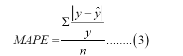
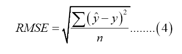
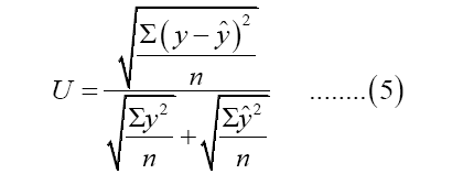
Where y is the actual inflation rate, y ̂ is the forecasted inflation rate, and n is the number of observations. The closer the values to zero, the better the forecasts.

Results and Discussion

A clear assessment of the plot in Figure 1 shows the existence of trend, a cyclical and seasonal variation, which indicates that, the series in non-stationary. The monthly mean plot in Figure 2 verifies the seasonality observed in the first plot. To achieve stationarity, the series is transformed to its natural logarithm. Further, seasonal differencing of the log series produces series diff (log (Inflation)) (see Figure 3). With no trend, non-seasonal differencing is no longer necessary.

Figure 1: Monthly Inflation in the Philippines January 2015- March 2020.

Figure 2: Means of Inflation by Month.

Figure 3: Differenced Log Series.

SARIMA models

The ACF of the differenced Inflation series in Figure 4 shows negative spike at lag 12 and 24, and a positive spike at lag 36. The PACF shows a positive spike at lag 12, revealing a possible seasonal MA of order one.

Figure 4: ACF and PACF of the Differenced Log Series.

For non-seasonal components, ACF decays slowly starting at lag 1 while PACF cuts off at lag 2. This tells us of the non-seasonal component of the model. With this, seasonal models and their orders are the following:

ARIMA (0, 1, 0) (1, 1, 0) (12)

ARIMA (2, 0, 0) (2, 1, 0) (12)

ARIMA (2, 0, 0) (1, 1, 0) (12)

Choosing the best model

The ARIMA (0, 1, 0) (1, 1, 0) (12) results in Figure 5 shows residuals of the model are normally distributed. The ACF of the model shows a spike at 18 but p-values from Ljung-Box statistics says that it is insignificant. Further, coefficient of seasonal component is significant (see Table 1).

Figure 5: Residuals of ARIMA (0, 1, 0) (1, 1, 0) (12).

The residuals from ARIMA (2, 0, 0) (2, 1, 0) (12) are shown in Figure 6. There are a few significant spikes in the ACF, and the model fails the Ljung-Box test. The model can still be used for forecasting, but the prediction intervals may not be accurate due to the correlated residuals. Coefficients of a non-seasonal and seasonal AR (1) are significant but constant is not (see Table 1).

Table 1. Summary of Fitted Models.

Figure 6: Residuals of ARIMA (2, 0, 0) (2, 1, 0) (12).

In Figure 7, residuals of ARIMA (2, 0, 0) (1, 1, 0) (12) shows a normal distribution. However, the ACF shows significant spike at lag 18 and some p-values from Ljung-Box test are insignificant. This result means that some data values are autocorrelated. Coefficients of a non-seasonal and seasonal AR (1) and the constant is significant (Table 1).

Figure 7: Residuals of ARIMA (2, 0, 0) (1, 1, 0) (12).

The best fitted model among the three models is ARIMA (0, 1, 0) (1, 1, 0) (12), having the lowest AIC and BIC values (Table 1). It has a significant coefficient, with no constant. Though the second model has the lowest MAPE, the best fitted model has a low MAPE value of 1.189417, which means that it has 98.81058% accuracy.

Forecasting

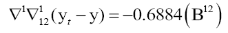
The final model for forecasting inflation is ARIMA (0, 1, 0) (1, 1, 0) (12) with the equation,

The model has a Mean Absolute Percentage Error (MAPE), Root Mean Square Error (RMSE) and Theil Inequality Coefficient value of 1.189417, 1.012582, and 0.089779, respectively (see Table 1). With the MAPE value, the model has an accuracy of 98.81058% for short-term forecast. Further, RMSE and Theil Coefficient are close to 0 which means that the model can be adequate in forecasting future values of Inflation.

The 24-month forecast of Inflation rates in the Philippines using the model are given in Table 2. Figures 8 and 9 further shows the forecasted data and the training set, and the forecasted data and the test set, respectively.

Table 2. Forecast for Inflation Rates.

Figure 8: Forecasted vs. Training set data.

Figure 9: Forecasted vs. Test set data.

Conlcusion

The monthly All-items Inflation rates in the Philippines have been shown to follow a seasonal ARIMA (0, 1, 0) (1, 1, 0) (12) which has been tested to be adequate. Using the model, 24-month forecast were produced with high accuracy. For future research, other inflation formulas are recommended to be used. Other factors such as the COVID-19pandemic can also be included as intervening variables to predict future prices.

References

1. Yap J. Inflation and Economic Growth in the Philippines. Philippine Institute for Development Studies. 2000

   [Google Scholar]

2. Philippine Statistics Authority. Inflation Report. 2020.
3. Tassew D. T. The Impact of Inflation to the Living Standard of Households. Int j economics commerce manag. 2015; 5:1-16.
4. Pidun u, et al. Why Companies Should Prepare for Inflation. The Boston Consulting Group. 2010.

   [Google Scholar]

5. Islam N. Forecasting Bangladesh Inflation through Econometric Models. Am. J. Econ. Bus. Adm. 2017; 9: 56-60.

   [Crossref] [Google Scholar]

6. Fritzer R, et.al. Forecasting Austrian Inflation. Economic Modelling. 2004; 24:470-480.

   [Crossref] [Google Scholar]

7. Bokhari, et.al. Forecasting Inflation through Econometric Models: An Empirical Study on Pakistani Data. Dogus Universitesi. 2006.

   [Google Scholar]

8. Sulekha A, et al. Impact of Inflation of the Household Spending Power. Int J Recent Technol Eng. 2019; 7:1-4.
9. Abdalla MM. Inflation Determinants in Sudan 1970-2009. Khartoum, Sudan: Central Bank of Sudan Publications. 2010.
10. Abdulrahman BMA. et.al. Forecasting of Sudan Inflation Rates using ARIMA Model. Int J Econ Finance. 2018; 8: 17-22.

    [Google Scholar]

11. Briner R.Is Inflation Dead? The Parthenon Group.1999.

    [Google Scholar]

12. Gujarati N, et al. Basic Econometric. McGraw-Hill, New Delhi. 2003.

    [Google Scholar]

13. Kuhe A, et al. Modelling and Forecasting CPI Inflation in Nigeria: Application of Autoregressive Integrated Moving Average Homoskedastic Model. J Sci Eng Res. 2016; 3: 57-66.  

    [Google Scholar]

14. Mankiw N.G.  Principles of Economics. 7th ed. USA: Cengage Learning. 2015.

    [Google Scholar]

15. Shiller R. J. “Why do people dislike inflation?” National Bureau of Economic Research, Inc. NBER Working Papers. 1996.

    [Google Scholar]

16. Inflation and Economic Growth in the Philippines