Keywords
|
| Dynamic reduction, coherency, aggregation, power system stability. model reduction, sub-optimal control. |
INTRODUCTION
|
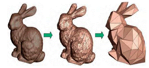
| Model Order Reduction always tries to quick capture the essential features of a structure. It means that is an early stage of the process, the basic properties of the original model must be present in the smaller approximation. At a certain moment the process of reduction should be stopped. So at that point all necessary properties of the original model must be captured with sufficient precision. All of this keep to be done automatically. Figure 1 illustrates the concept in a graphical way to understand the Model Order Reduction[24]. It demonstrates that sometimes very little information is needed to describe a model. |
| This example with pictures of the Stanford Bunny shows that, even with only a few facets, the rabbit can still be recognized. Although this example is constructed for an entirely different purpose, and does not contain any reference to the way model order reduction is performed mathematically. This paper is organize as follows: Section I give the introduction of the Model Order Reduction. Section II is helpful to understand the reduction process. Section III explains the system modeling in terms of stability. Section IV shows the design specification of the 4th order system. Section V conclude the paper and followed by the references |
RELATED WORK
|
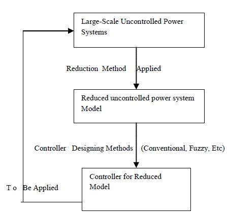
| Figure 2 shows the process of Model Order Reduction as every physical system can be translated into mathematical model. The mathematical procedure of system modeling often leads to comprehensive description of a process in the form of high order differential equations which are difficult to use either for analysis or controller design. It is therefore useful, and sometimes necessary to find the possibility of finding some equations of the same type but of lower order that may be considered to adequately reflect the dominant properties of the high order system. Some of the reasons for using reduced order models of high order linear systems could be |
| ïÃâ÷ To reduce computational complexity. |
| ïÃâ÷ To reduce hardware complexity. |
| ïÃâ÷ To have a better understanding of the system. |
| ïÃâ÷ To design efficient controllers. |
| ïÃâ÷ To use the reduced order system economically for on-line implementation. |
THE DYNAMIC REDUCTION PROCESS
|
| To place model reduction in a mathematical context, we require to realize that many models developed in computational science consist of a system of partial or ordinary differential equations, supplemented with boundary conditions. Important examples are the Navier-Stokes equations in computational fluid dynamics (CFD), and the Maxwell equations in electromagnetic Theory. When partial differential equations are to be used to describe the behavior, one often encounters the situation that the independent variables are time and space. Thus, after discrediting in space, a system of ordinary differential equations is obtained in time. Therefore, we limit the discussion to ODEâÃâ¬ÃŸs and consider the following[24] explicit finite-dimensional dynamical system |
 |
 |
| where the dimension of ˆx is much smaller than n. In order to provide a good approximation of the original input-output system, a number of conditions should be satisfied: |
| ïÃâ÷ the approximation error is small, |
| ïÃâ÷ preservation of properties of the original system, such as stability and passivity, |
| ïÃâ÷ the reduction procedure should be computationally efficient. |
| A special case is encountered if the functions f and g are linear, in which case the system reads |
 |
 |
| Here, the matrices A,B,C,D can be time-dependent, in which case we have a linear time-varying (LTV) system, or time-independent, in which case we speak about a linear time-invariant (LTI) system. For linear dynamical systems, model order reduction is equivalent to reducing the matrix A, but retaining the number of columns of B and C. |
| The process to reduce the dynamic model of a power system can be divided into three stages: coherency identification, generator aggregation, and network reduction. |
A. COHERENCY IDENTIFICATION
|
| In this stage, coherent generators are identified and grouped together. This identification procedure may be greatly simplified [3] by using the following assumptions: |
| ïÃâ÷ non-generator dynamics may be ignored |
| ïÃâ÷ classical generator models may be used |
| ïÃâ÷ the linearized system model preserves well the trends of coherency |
| Under these assumptions, the system model can be represented in a linear state space form. |
 |
| where the dimension of the state matrix A corresponds to the number of generators in the system, and the state vector X contains generator speeds only. |
B. GENERATOR AGGREGATION
|
| After a group of coherent generators is identified[3], the generators in it are aggregated and reduced to one or a few equivalent generators. Generally, the generator aggregation can take one of two forms: |
ïÃâ÷ CLASSICAL AGGREGATION (CA)
|
| The generators in a coherent group are represented by an equivalent classical generator model. In its simplest form, the equivalent inertia is the sum of the inertia of all generators in the group, and the equivalent transient reactance is obtained by paralleling the transient reactance of all generators in the group[10]. |
ïÃâ÷ DETAILED AGGREGATION (DA) [13]
|
| If some or all generators in a coherent group have similar control systems, they can be aggregated to a detailed generator model with an equivalent exciter, stabilizer, and governor. The parameters of the equivalent models are obtained using a combination of two approaches: a least square fit of the frequency responses to determine the linear characteristics, and an evaluation of the time-domain constraints to set the nonlinear characteristics. |
C. NETWORK REDUCTION
|
| Once equivalent generators are determined for the coherent groups, a network reduction is performed. This reduction is achieved in two steps: |
| ïÃâ÷ The equivalent generators are inserted into the system and the generators in the associated coherent groups are removed. The network is modified to maintain the balanced steady state power flow conditions. |
| ïÃâ÷ The network is reduced by using an adaptive reduction technique similar to the one in [14], which automatically determines the buses to be eliminated such that maximum advantage is taken of network sparsity. |
SYSTEM MODELLING IN TERMS OF STABILITY
|
A. STABILITY
|
| Poles and Eigen values of a system are strongly related to the stability of the system. Stability is the property of a system that ensures that the output signal of a system is limited (in the time domain). Consider, The system is stable if and only if, for all Eigen values λj , we have that Re(λj) ≤ 0, and all Eigen values with Re(λj) = 0 are simple. In that case, the corresponding matrix A is termed stable, There are several properties associated with stability. Clearly, if A is stable, then also A−1 is stable. Stability of A also implies stability of AT and stability of A*. |
| Finally, if the product of matrices AB is stable, then also BA can be shown to be stable. It is also clear that, due to the relation between Eigen values of A and poles of the transfer function, stability can also be formulated in terms of the poles of H(s).The more general linear dynamical system- |
 |
 |
| is stable if and only if for all generalized Eigen values we have that Re(λj(Q,A))≤ 0, and all generalized Eigen values for which Re(λj(Q,A)) = 0 are simple. The set of generalized Eigen values σ(Q,A) is defined as the collection of Eigen values of the generalized Eigen value problem. |
 |
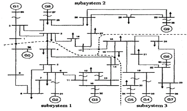
| In this case, the pair of matrices (Q,A) is termed a matrix pencil. This pencil is said to be regular if there exists at least one Eigen value λ for which Q + λA is regular. Just as for the simpler system discussed in the above, stability can also be formulated in terms of the poles of the corresponding transfer function. Here Eigen values of the reduced state equation are estimated [18]. New England 10- generator 39-bus system is used. New England 10-generator 39-bus system is shown in Fig. 4. In this case, the whole system is divided into three areas. It is considered that the oscillation modes which should be reserved are 0.6- 6.O[Hz] frequency modes. Since the reduced modes are considered to be sufficiently fast modes, selection of reduced mode should be mode considering Eigen values. In the case, if the absolute value of the Eigen value is larger than the threshold, corresponding mode is reduced. |
| Three model reduction methods are used as follows. |
| ïÃâ÷ the model reduction method 1: the reduced mode xi2 is made equal to zero. |
| ïÃâ÷ the model reduction method 2: the reduced mode xi2 is represented as |
 |
| ïÃâ÷ the model reduction method3: the reduced mode xi2 is represented as |
 |
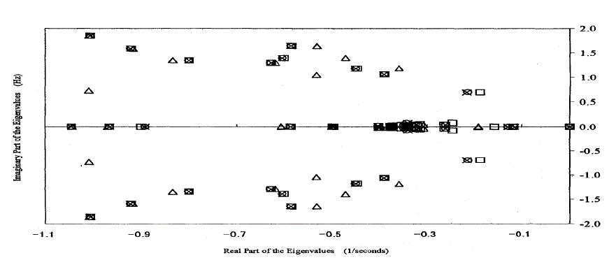
| The Eigen values of original and reduced system is shown in Fig, 5. „The numbers of oscillation modes in subsystems are reduced as follows |
| subsystem 1 : 30 → 18 |
| subsystem 2 : 30 → 18 |
| subsystem 2 : 30 → 18 |
| The number of oscillation modes in the aggregated system becomes 60 in this case. Since the system is stable, all real part of Eigen values is negative. However,positive real part. On the contrary, using the model reduction method 2 or 3, real part of every Eigen value stays negative. using the model reduction method 1, a pair of the complex Eigen values has |
| The difference between the method 2 and the method 3 can be recognized in Table 3. Each Eigen values obtained by the method 3 is closer to that of the original system. |
B. STABILITY CONSTRAINTS POLYNOMIALS
|
| The most general constraints are easily tractable by concurrent software like Linear Matrix Inequalities (LMIs). So, we search for LMIs ensuring stability of linear in parameters systems[20]. For considering fixed-coefficients system stability is the first step. To the best of our knowledge, the most advanced LMI characterization of stability domain in coefficients space of polynomial is SPR rational function based LMI characterization [10] and its improvement [11]. The SPR-based method [10] states that F(z) is stable if for some stable d(z) and any (small) η |
 |
| This inequality can be derived by noting that stability of F(z)is equivalent to existence of stable polynomial d(z) such that F(z)/d(z) is Strictly Positive Real. The above difference is formulated in [10] as LMI. |
| This paper propose to choose the “central polynomial” in an iterative way, suitable for our problem of model reduction. First we start with a stable polynomial (better to be close to the optimal one), for example, the “central polynomial” of [10] or [11]. Then we perform model reduction with stability-ensuring LMI constraints [10] built with this polynomial. The resulting reduced model is taken as the new “central polynomial” and the process repeats until no improvement in model reduction error is seen |
| C. STABILITY CONSTRAINTS FOR INTERVAL POLYNOMIALS In case we seek for uncertain ˜ f(z) (i.e. interval polynomial), each “vertex polynomial” should be constrained by the same LMI. Since LMI is convex, this way we ensure that the whole interval polynomial is stable. |
DESIGN SPECIFICATION
|
| Here we have consider a4th order system[6], |
 |
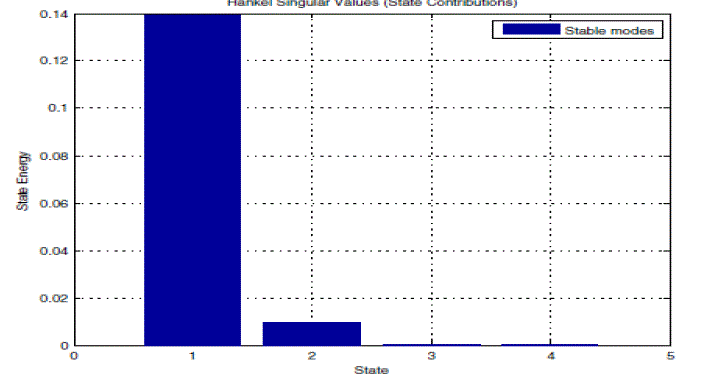
| The given 4th order system is reduced to 1st, 2ndand 3rd order by using BTR algorithm. By graphical analysis good approximation between reduced and original model is obtained. A plot of the Henkel Singular Values is obtained and then less dominant states of the system are predicted. These states do not have much impact on input-output behavior. These states are eliminated to obtain reduced order model. |
| From fig.6 we can predict that state 1 having maximum singular value and having maximum impact on systems behavior. Other three states which have less magnitudes can be eliminated to obtain reduced order model. Error bound on the difference in frequency response between that of the original system and the reduced order system is applied for verification. |
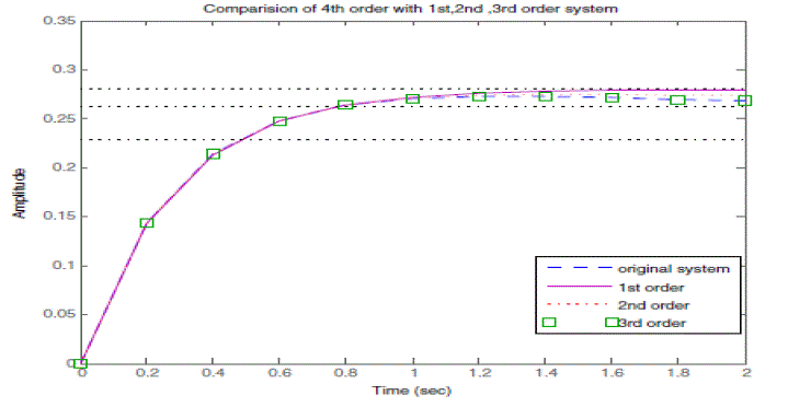
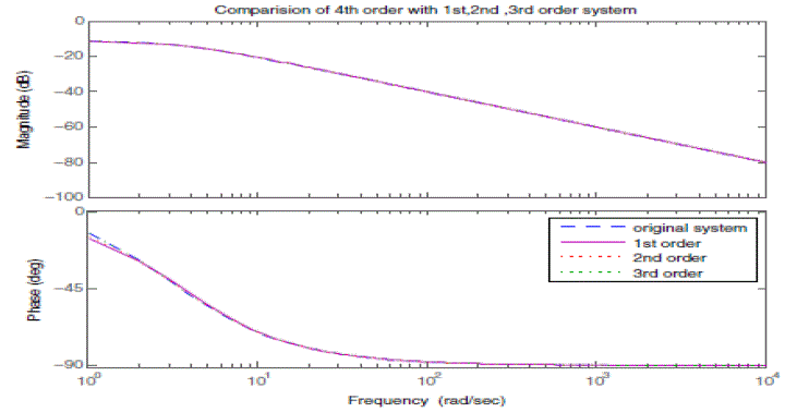
| Now the original system is reduced to 1st, 2nd, and 3rd order. The response of the original system is compared with 1st,2nd, and 3rd order system by using step response and bode plot as shown in figure (9) and figure (10).For 1st order model, The resulting upper-error bound is |
 |
| For 2nd order model, the resulting upper-error bound is |
| 2*(0.0000+0.0000) = 0.0000 |
| thus by selection of acceptable error limit and the reduced order model by choosing approximation order r is obtained. The step response and bode plot of original and various reduced order systems are as shown in figure (8) and figure (9). |
| From figure (7) and (8), it is concluded that reduction of less dominant states does not make much difference in system behavior and shows good match of response and error within acceptable limit. |
CONCLUSION
|
| We have reviewed the most important methods for model order reduction. The discussion is certainly not comprehensive, alternative methods have been published. For example, we have not mentioned the methods of Arnoldi and PRIMA, Laguerre, Optimal Hankel Norm Reduction and Proper Orthogonal Decomposition etc. These methods build rational approximations of the transfer function in a very intellectual and efficient way, and can be used to adaptively put together reduced order models. As we have described model order reduction is a very active area of research, progress in this very active area may lead to an exclusively new category of methods. The enlargement of such new methods is often sparked by an industrial need. For example, right now there is a require for dipping problems in the electronics production that contain numerous inputs and outputs. It has already become clear that current methods cannot cope with such problems, as the Krylov spaces very swiftly become inhibitive great, even after a few iterations. for this reason, new habits of constructing reduced order models must be developed. The problem of ensuring stability is shown during model reduction of interval linear-in-parameters systems. The stability constraints are also formulated in form of LMI. |
| As planning or operating stability studies[3], large power system models can be reduced by up to 50% with no extreme loss of accuracy. The three coherency identification methods considered in this paper all produce good generator grouping. No major difference in the quality of the reduced models was observed by using these three poles apart methods. Classical aggregation of coherent generating units fallout in simpler and lower order reduced models than detailed aggregation and is adequate in many cases. In some cases, a detailed aggregation is required to realize improved accuracy. The accuracy of a reduced order model, with respect to a definite observable fact, depends to a great extent on retaining the system elements which are most applicable to that phenomenon. It is therefore essential to have a considerate of the phenomenon before starting the reductions. A reduced model of a power system that is appropriate for the study of one phenomenon in that system is not essentially suitable for the study of another phenomenon |
Tables at a glance
|
 |
| Table 1 |
|
Figures at a glance
|
 |
 |
 |
 |
| Figure 1 |
Figure 2 |
Figure 3 |
Figure 4 |
 |
 |
 |
 |
| Figure 5 |
Figure 6 |
Figure 7 |
Figure 8 |
|
References
|
- Y. Mansour, E. Vaahedi, A.Y. Chang, B.R. Coms, B.W.Garrett, K. Demaree, T. Athay, K. Cheung, “B.C. HydroâÃâ¬ÃŸs On-line Transient StabilityAssessment (TSA) Model Development, Analysis, and Post-processing”, IEEE Trans.Vol. PWRS-10, pp. 241-253, February, 1995.
- J.H. Chow, R. Galarza, P. Accari, and, W.W. Price, “Inertial and Slow Coherency Aggregation Algorithms for Power System Dynamic ModelReduction”, IEEE Trans. Vol. PWRS-IO, pp. 680-685, May, 1995.
- Lei Wangt, Meir Klei, Solomon YirgatandPrabhaKundurt “Dynamic Reduction of Large Power Systems for Stability Studies” IEEE Transactions onPowcr Systems, Vol. 12, No. 2, May 1997.
- Nelson Martins, Julio C. R. Ferraz, Paulo E.M. Quintão,Alex De Castro, Sergio. Varricchio, Sergio Gomes Jr. “Linear Techniques Applied To Small-Signal Electromechanical Stability, Model Order Reduction And Harmonic Studies” Intelligent Automation and Soft Computing, Vol. 12, No. X, pp. 1-13,2006.
- Mittal A. K., Sharma S. P and Prasad R., “Reduction of multivariable systems using the advantages of Mihailov criterion factor division”, Proc.International Conf. on Computer applications in Electrical Engg., Recent advances, Indian Institute of Technology, Roorkee, India, pp. 477-482,Feb. 2002.
- Poonam J. Patil and Mukesh D. Patil* “Model Order Reduction Of High Order LTI System using Balanced Truncation Approximation””, IETE Journal ofResearch, Vol. 53, No. 2, pp. 98-102, March-April 2007.
- Prasad R. and Pal. J., “Stable reduction of linear systems by continued fractions”, Journal of Institution of Engineers India, IE (I) journal –EL, Vol. 72,pp. 113-116, 1991.
- Parmar G., Mukherjee S. and Prasad R., “Model reduction with time delay using Cauer second form”, Proc. Second National Control InstrumentationSystem Conference (CISCON-2005), Manipal Institute of Technology (MIT), Manipal, India, pp. 150-153, November 11-12, 2005.
- Parmar G., Prasad R. and Mukherjee S., “Reduction of linear dynamic systems using dominant pole retention method and modified cauercontinuedfraction”, Journal of Computer Science (JCS), Karpagam Publication, India, Vol. 1, No. 6, pp. 547-554, 2006
- Vishwakarma C. B. and Prasad R., “Reduced order modelling using pole clustering and cauer second form”, CD-R Proc. National Conference on RecentAdvances in Electrical Engineering (RAEE-2008) , National Institute of Technology, Hamirpur, India, December 26-27, 2008.
- Pade H., “Sur La representation approaches dune function pardes fractions rationelles”, AnnalesScientifiquesdeâÃâ¬ÃŸlEcoleNormaleSupieureSer 3 (Suppl)9, pp. 1-93, 1892.
- Prasad R. and Devi S., “Reduction of discrete multivariable systems using Pade type modal methods”, Journal of Institution of Engineers India, IE (I)Journal-EL, Vol. 82, pp. 72-77, 2001.
- A.J. Germond and R. Podmore, “Dynamic Aggregation of Generating Unit Models”, IEEE Trans. Vol. PAS-97, pp. 1060- 1069, July/August, 1978.
- W.F. Tinney and J.M. Bright, “Adaptive Reductions for Power Flow Equivalents”, IEEE Trans. Vol. PWRS-2, pp.351-360, May 1987.
- Singh Nidhi, Prasad R. and Gupta H. O., “Reduction of power system model using Balanced realization, Routh and Pade approximation methods”,International Journal of Modelling and Simulation, Acta Press, Vol.28, No. 1, pp. 57-63, 2008.
- Vishwakarma C.B and Prasad R., “System reduction using modified pole clustering and Pade approximation”, CD-R Proc. XXXII National SystemsConference, NSC-2008, Indian Institute of Technology, Roorkee, India, pp. 592-596, December 17-19, 2008.
- Vishwakarma C.B and Prasad R., “System modelling using improved Pade approximation and differentiation technique”, Proc. National Conference on ITResearch and Applications, Maharaja Agrasen Institute of Management and Technology, Jagadhary, Haryana, pp. 64-67, November 16-18 , 2007.
- Goro Nobuyuki Nihei Tsutomu Oyama “A Study on Decomposition and Model Reduction for Wide Area Power System Stabillity Assessment” 0-7803-4403-0/98, pp.651 1998 IEEE Mar20, 1998
- L. Fortuna, A. Gallo, G. Nunnari, Model Order Reduction Techniques with Application in Electrical Engineering , Springer-Verlag, October 1992
- H. Rotstein, N. Galperin, P.-O. Gutman, Set membership approach for reducing value sets in the frequency domain, IEEE Trans. AC, vol.43, no.9, pp.1346–1350, Sep. 1998
- B. Bandyopadhyay, O. Ismail and R. Gorez, Routh-Pade approximation for interval systems, IEEE Trans. Aut. Contr., Vol. 39, pp. 2454–2456,Dec. 1994.
- Y.Dolgin, E.Zeheb, Model reduction of uncertain systems: approximation by fixed-coefficients system, IEEE Trans. Aut. Control., vol. 51, pp. 406-411,2004.
- Y.Dolgin, E.Zeheb, Model reduction of uncertain systems retaining the uncertainty structure, Systems & Control Letters, Volume 54, Issue 8, pp. 771-779,2005
- (Eds.) W.H. Schilders; H.A. van der vorst; j. Rommes 2008, 8II, 472p. 133 illus., 53 in color, HardCOVER ISBN: 978-3-540-78840-9
- Vishwakarma C. B., and Prasad R., “Order reduction using the advantages of differentiation method and factor division”, Indian Journal of Engineeringand Material Sciences, Niscair, India, Vol. 15, No. 6, pp. 447-451, 2008.
- Parmar G., Mukherjee S. and Prasad R., “Relative mapping errors of linear dynamic systems caused by Genetically optimized reduced order model”,Journal of Computer Science (JCS), Karpagam, India, Vol. 2, No. 3, pp. 231-237, 2006.
- Parmar G., Mukherjee S. and Prasad R., “Relative mapping errors of linear dynamic systems caused by particle swarm optimized reduced order model”,Proc. Int. Conf. Intelligent Systems & Networks (IISN-2007), Computational Intelligence Laboratory , Jagadhary (Haryana), India, pp. 371-377, Feb. 23-25, 2007.
|