Pratap Kumar Jena*, Runu Lata Sahoo
Department of Economics, Maharaja Sriram Chandra Bhanjadeo University, Baripada, Odisha, India
Received: 01-Aug-2022, Manuscript No. JSS-22-70935; Editor assigned: 03-Aug-2022, Pre QC No. JSS-22-70935 (PQ); Reviewed: 17-Aug-2022, QC No. JSS-22-70935; Revised: 05-Oct-2022, Manuscript No. JSS-22-70935 (R); Published: 12-Oct-2022, DOI: 10.4172/JSS.8.6.001
Visit for more related articles at Research & Reviews: Journal of Social Sciences
The relationship between Foreign Direct Investment (FDI) and manufacturing output is being investigated by researchers at the international and national levels, and their findings are contradictory to each other. Although, some studies found a positive relationship between FDI and manufacturing output, and other studies found no relationship between these two variables. Some studies found the relationship but vary in the long-run and short run. Therefore, this paper has examined the nexus between FDI and Manufacturing Output Index (MFI) in India using the Auto Regressive Distributed Lag (ARDL) bounds test. The paper found the integration in both the long run and short run between FDI and MFI. Since the manufacturing sector is one of the important sectors in India for employment and economic growth, the government has to attract more FDI by providing certain facilities like; good environment for business investment, tax concessions, new investment opportunities in the manufacturing sector, etc.
FDI; Manufacturing output; Augmented ARDL; Economic growth
In recent years, India is one of the most eye-catching destinations for investments in the manufacturing sector in the world. Investment is crucial for industrialization in a country, due to inadequate domestic investment, Foreign Direct Investment (FDI) has been attracted to the industries to foster the manufacturing output, employment and economic growth. Developing countries have been trying to attract more FDI to different sectors. Besides that, the FDI enhances skills and advanced technology, productivity and standard of living in the long-run. The FDI has a spillover effect on the macroeconomic variables, which finally enhances economic growth. It has been recorded that the FDI has increased at a significant rate in the post-reform period and achieved new heights during the 20th century. India is ranked among the top 10 recipients of FDI in South Asia, which has attracted US $49 billion. The cumulative FDI in India’s manufacturing sector reached US $89.40 billion 2000 to 2020, and the govt. of India has increased FDI from 49% to 74% on defense manufacturing under the automatic route.
Policy makers and academic researchers at the international level have been examined the linkage between the FDI and manufacture output, but there is a lack of literature for India. Turkan, et al., and Agrawal have found a positive relation between FDI, manufacturing sector and economic growth. On the other hand, Oyatoye, et al. obtained a poor attraction of FDI to the Nigerian economy, and the FDI had little or no impact on the manufacturing capacity utilization in Nigeria. Afolabi, et al. analyzed the connection between the Nigerian manufacturing sector and FDI and found that the manufacturing out was influenced by FDI and other macroeconomic variables such as Inflation Rate (INF), Government Expenditure (GOE), and Money Supply (MSP). That is because the FDI in the manufacturing sector is negatively influenced by different factors such as; import-intensity, R&D intensity, and positively influenced by the market power. India is one of the most attractive destinations of FDI in the world, which can be achieved through quick project clearance, improving coordination between the states and the central government for project clearance is imperative by making SEZs more attractive, proper planning and design. The relationship between FDI, manufacturing sector and economic growth is inconclusive as studies derive different results [1].
From the existing studies, it is not clear on the relationship between Foreign Direct Investment (FDI) and the manufacturing sector in India, Therefore, this paper is examining the relationship between FDI and the manufacturing sector in India at a disaggregated level with emphasis on implications for capital formation in the sector and market structures. The rests of the paper are as follows; section-2 describes the composition, market size and performance of the manufacturing sector in India. Section-3 provides study variables and methodology. Section-4 discusses the estimated results, and the last section-5 provides the conclusion of the study [2].
Manufacturing sector in India: Composition, market size and performance
In pre independence, India was exporting huge quantities of manufacturing products, most of them were handicraft products that have been declined due to the regressive policies of the government. After independence, the government has implemented the industrial policy in 1956, and there was the development of basic and heavy industries such as iron & steel, heavy engineering, lignite projects, and fertilizer, etc. The new economic policy has increased the competition of domestic products in the international markets [3].
The India Brand Equity Foundation (IBEF) has categorized the manufacturing industries based on size, and use of inputs or raw materials. The size of manufacturing industries depends on capital investment, workers employed and quantities production, such industries are household or cottage industries (includes bamboo, leather, wood, bricks, fabrics, stones, mud materials, etc.), small scale manufacturing industries (workshop outside home or cottage production), and large scale manufacturing industries (includes superior technology, large capital, large production, etc). The second type of classification was based on the use of inputs or raw materials, and such industries are agro based industries (includes rural and urban businesses like; food processing, fruits juices, pickles, beverages, cotton, silk, etc.), food processing (includes the production of cream, canning, confectionary, and fruits), mineral based industries (includes iron and steel industries and non-ferrous metallic minerals like cooper, aluminium and jewellery, etc), chemical based industries (like sulphur, potash, synthetic fibre, plastics, etc.), forest based raw material using industries (includes; minor and major forest products, wood and grass, etc.), and animal based industries includes leather and wool industries, etc.
Market size and performance: India has ranked 30th in the global manufacturing index in 2018, and the Gross Value Added (GVA) of the manufacturing sector at basic prices was US$ 403.23 billion in the financial year 2019. The Compound Annual Growth Rate (CAGR) of GVA in manufacturing sector was recorded at 4.29% during the financial year 2012-19. The Index of Industrial Production (IIP) of manufacturing sector grew at 3.50%, where the high growth rate was recorded in the production of basic metals, intermediate goods, food products, and tobacco products. The Gross Fixed Capital Formation (GFCF) or net investments in fixed assets was US$, 405.88 billion in 2019-20, and was expected that it may touch US $1 trillion by the end of 2025 [4].
It has been observed that the contribution of the manufacturing sector to India's GDP was 6.8% in 2018, whereas, the contribution to world GDP was 3%, which suggests that the manufacturing sector has a significant contribution to the national income of India. The growth rate of the manufacturing sector and the economic growth rate during 1991 to 2018 are reported in Figure 1, which indicates that both growth rates have fallen after 2007 and have more volatility, but FDI is more volatile than the GDP growth rate in the study period, that makes worrisome to the policymakers in India. The manufacturing output has various uses, which is broadly categorized into six uses such as primary goods (34%), capital goods (8%), intermediate goods (17%), infrastructure/construction goods (13%), consumer durables (13%) and consumer non-durable goods (15%). It indicates that the manufacturing outputs are largely used as primary goods followed by intermediate goods, and the least output is used in capital goods in India (Figure 2).

Figure 1: Trends of FDI and manufacturing sector in India during 1991-2018.
Source: Authors estimation by using RBI database data.

Figure 2: Uses of manufacturing output in India.
Source: Authors estimated
Figure 3 draws the picture of Gross Value Added and Employment growth rate of manufacturing industries from 1987-88 to 2017-18. And found that GVA has been rising steadily over the years witnessing a growth rate of 62.8% in 2017-18. The growth rate of employment has been relatively lower i.e. 3.8% in 2017-18.

Figure 3: Trends of GVA and employment in the manufacturing sector in India.
Source: Authors estimated
The Compound Annual Growth Rate (CAGR) of major manufacturing product industries in India during the period 2012-13 to 2017-18 is reported in Table 1. It shows that the tobacco products industry has the highest CAGR (2.48%), followed by other manufacturing industries (1.27 percent) and electrical equipment (1.02 percent). The wood, and products of wood and cork, except furniture of articles had a positive CAGR (0.98 percent). All other manufacturing industries have a negative compound growth rate but the pharmaceutical, medicinal products, and botanical products, and furniture had a larger negative CAGR during 2012-13 to 2017-18 in India [5-9].
| Industry group | 2012-13 | 2017-18 | CAGR (2012-13 to 2017-18) |
|---|---|---|---|
| Food products | 103.3 | 108.1 | -0.90% |
| Beverages | 106.7 | 105.4 | 0.25% |
| Tobacco products | 107.5 | 95.1 | 2.48% |
| Textiles | 108 | 117.1 | -1.60% |
| Wearing apparel | 99 | 137.5 | -6.36% |
| Leather and related products | 110.6 | 123.9 | -2.25% |
| Wood and products of wood and cork, except furniture of articles | 97 | 92.4 | 0.98% |
| Paper and paper products | 103.3 | 108.9 | -1.05% |
| Printing and reproduction of recorded media | 96.8 | 99.7 | -0.59% |
| Coke and refined petroleum products | 105.9 | 123.5 | -3.03% |
| Chemicals and chemical products | 103.9 | 116 | -2.18% |
| Pharmaceuticals, medicinal chemical, and botanical products | 108.1 | 212.1 | -12.61% |
| Rubber and plastic products | 101 | 110.6 | -1.80% |
| Other non-metallic mineral products | 102.9 | 113.9 | -2.01% |
| Basic metals | 107.8 | 138 | -4.82% |
| Fabricated metal products, except machinery and equipment | 97 | 107.9 | -2.11% |
| Computer, electronic and optical products | 100.6 | 148.5 | -7.49% |
| Electrical equipment | 113 | 107.4 | 1.02% |
| Machinery and equipment | 102.9 | 120.5 | -3.11% |
| Other transport equipment | 99.2 | 133.9 | -5.82% |
| Motor vehicles, trailers and semi-trailers | 100.1 | 114.5 | -2.65% |
| furniture | 112.9 | 196.6 | -10.50% |
| Other manufacturing | 113.1 | 106.2 | 1.27% |
| Manufacturing | 104.8 | 126.6 | -3.71% |
| Source: Hand book of statistics, RBI |
Table 1: Compound annual growth rate of major manufacturing industries in India.
The relationship between FDI and the manufacturing sector in India has been examined using the time series data, collected from the handbook of statistics on the Indian Economy, the Reserve Bank of India (RBI), and the National Sample Survey Organization (NSSO) database. The study selected variables are the Index of Manufacturing Sector (IMS) and FDI collected from 1991 to 2019 [10-15].
To examine the relationship between FDI and manufacturing output in India, the study has employed the ARDL model proposed by McNown et al. Though there are various co integration techniques such as Johansen, Engle-Granger, and Johansen-Juselius available, which assumed a unique order of integration, whereas the ARDL model is more flexible in terms of order of integration? This model is applied if the study time series variables are of a different order of integration such as I (0) and I (1), but not applicable to variables of I (2). Moreover, it gives more options for the lag selection of variables and handles the endogeneity of variables, if any exist. McNown, et al. proposed ARDL model is an upgraded version of the Pesaran, et al. model, known as augmented ARDL, which is necessitated an additional t-test or F-test for significance level [16-18].
The ARDL model is as follows:
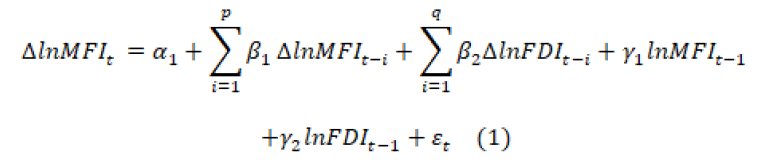
Where, α1 is an intercept term, εt is a white noise error term and, Δ is a first difference operator. The summation terms indicate short-term dynamic relations, whereas, the terms with αs shows the long-term dynamic relations between the selected variables. Here, the null hypothesis is γ1= γ2=0, which means there is no integration or long run relationship between the study variables that can be examined using the F-Test and t-test proposed by McNown, et al. If the estimated F-stat is greater than the upper bound critical value, then the null hypothesis is rejected, which implies a long run relationship exists between the variables. On the other hand, if the estimated F-stat is neither lower nor greater than the two critical values, then the relationship between variables is inconclusive [19].
The short run dynamic relationship between study variables is examined using the Error Correction Model (ECM) as follows:

Where, the δs indicates the short run dynamic coefficients, the ECT is the error correction term and θ shows the speed of adjustment, which lies between 0 to -1, where, 0 implies no convergence towards equilibrium, and -1 indicates a perfect convergence. The stationary condition of the study variables has been checked by using the unit root tests such as Augmented Dickey and Fuller (ADF) test and Phillips Peron (PP) test. The variables natural logarithmic values have been used in the analysis [20-23].
The manufacturing output is one of the important components of the Index of Industrial Production (IIP) is recorded at 129.8 in the year 2020, which seems very strong in the production of basic metals (10.8%), intermediate goods (8.8%), food products (2.7%) and tobacco products (2.9%) (RBI online database). If we look at the trends of FDI and MFI during 1991 and 2019 as shown in Figure 4, indicate that both the trends of FDI and MFI are rising upward, but the FDI trend is raising upward faster than the MFI trend. The FDI trend is highly fluctuating than the MFI trend in the study period.

Figure 4: Trends of FDI and manufacturing sector in India during 1991-2018.
Source: Authors estimation by using RBI database data.
The descriptive statistics of FDI and MFI variables indicate that both the mean and standard deviation values of FDI are higher than the MFI, which indicates the foreign direct investment has a higher average value and volatility in India in the study period (Table 2). The skewness values are negative, the kurtosis and Jarque-Bera values indicate the normal distribution of variables. The correlation coefficient value is 0.94 indicates a high positive correlation between FDI and MFI during the study period in India (Table 3).
| LNMFI | LNFDI | |
|---|---|---|
| Mean | 4.066 | 10.437 |
| Std. Dev. | 0.586 | 2.015 |
| Skewness | -0.122 | -0.935 |
| Kurtosis | 1.567 | 3.330 |
| Jarque-Bera | 2.553 | 4.358 |
| Probability | 0.279 | 0.113 |
| Observations | 29 | 29 |
| Source: Authors estimation | ||
Table 2: Descriptive statistics of FDI and MFI in India.
| LNMFI | LNFDI | |
|---|---|---|
| LNMFI | 1 | 0.94 |
| LNFDI | 0.94 | 1 |
| Source: Authors estimation | ||
Table 3: Result of correlation coefficient.
The estimation of a time series model needs optimal lag length, which is selected through the lag length selection criteria and the estimated results are reported in Table 4. It indicates that the lag selection criterion indicates that one is the optimum lag, which is used for the model estimation.
| Lag | LogL | LR | FPE | AIC | SC | HQ |
|---|---|---|---|---|---|---|
| 0 | -28.28136 | NA | 0.032302 | 2.243064 | 2.339052 | 2.271606 |
| 1 | 57.06774 | 151.7317* | 7.82e-05* | -3.782796* | -3.494832* | -3.697169* |
| 2 | 60.07431 | 4.899584 | 8.47e-05 | -3.709208 | -3.229268 | -3.566497 |
| *Indicates lag order selected by the criterion LR: sequential modified LR test statistic (each test at 5% level) FPE: Final Prediction Error AIC: Akaile Information Criterion SIC: Schwarz Information Criterion HQ: Hannan_Quinn information criterion |
||||||
Table 4: Results of optimal lag length.
The stationary conditions of both the study variables are checked by using the unit root tests such as ADF and PP, the results are reported in Table 5. It shows that FDI is stationary at the level values, whereas, the MFI is non-stationary at the level values but becomes stationary at the first difference in both intercepts, and intercept with the trend. Although the study variables are a mix of I (0) and I (1), the relationship between these variables is measured using the ARDL model bound test, the results are reported in Table 6.
| The estimated t-statistics values from Unit root (level) | ||||
|---|---|---|---|---|
| Intercept alone | Intercept + Trend | |||
| ADF | pp | ADF | pp | |
| LNMFI | 1.89 | 1.29 | -2.29 | -2.2 |
| LNFDI | -4.63* | -4.63* | 4.85* | -4.95* |
| The estimated t-statistic values from unit root test (First difference) | ||||
| LNMFI | -3.27** | -3.26** | -3.45*** | -3.51*** |
| Notes: a. Critical values for unit root test (ADF and DF) are -3.69 (1%), -2.97 (5%) and -2.62 (10%) without trend and -4.37 (1%), -3.60 (5%) and -3.24 (10%) with trend. And for DF test critical values are -2.66 (1%), -1.95 (5%) and -1.60 (10%) without trend and -3.77 (1%), -3.19 (5%) and -2.89 (10%) with trend. b. *,** and *** indicates stationary respectively at 1%, 5% and 10% levels. Source: Authors computation using E-views 10 student version. |
||||
Table 5: Results of unit root test.
The ARDL bound test results indicate that the estimated F-stat value (54.09) is higher than the upper bound critical value at 1% level that means the existence of a long run relationship between FDI and MFI in the study period. The ARDL model lag order is selected through the AIC that suggests the ARDL (1, 0) model is a better order than others (Table 6).
| Critical value | F-Statistics | Lower bound value | Upper bound value |
|---|---|---|---|
| 10% 5% 2.50% 1% |
54.09 | 3.02 3.62 4.18 4.94 |
3.51 4.16 4.79 5.58 |
| Source: Authors estimated | |||
Table 6: Result of bound test.
The ARDL model results are reported in Table 7, which indicates all coefficients are significant at the 1% level. The cointegration results indicate the long run cointegration between FDI and MFI. To support the long run cointegration between the study variables, we have estimated the short-term cointegration using the ARDL-VEC model, the results are reported in Table 8. The ECM coefficient value -0.18 is significant at the 1% level, which means there is a short-term relationship between the FDI and MFI. Hence, the present study has found that the existence of both short-run and long-run cointegration between FDI and MFI during the study period.
| Conditional error correlation regression | ||||
|---|---|---|---|---|
| Variable | Coefficient | Std. Error | t-Statistic | Prob |
| C | 0.165155 | 0.040141 | 4.114396 | 0.0004 |
| LNIMS(-1)* | -0.181469 | 0.032165 | -5.641720 | 0.0000 |
| LNFDI** | 0.059081 | 0.010615 | 5.565816 | 0.0000 |
| *P-value incompatible with t-Bounds distribution. **Variable interpretend asZ=Z(-1)=D(Z) |
||||
| Levels equation Case 2: Restricted constant and no trend |
||||
| Variable | Coefficient | Std. Error | t-Statistic | Prob. |
| LNFDI | 0.325571 | 0.017289 | 18.83099 | 0.0000 |
| C | 0.910101 | 0.189563 | 4.801059 | 0.0001 |
| EC=LNIMS=(0.3256*LNFDI=0.9101) | ||||
Table 7: ARDL long run model.
| ECM Regression Case 2: Restricted constant and no trend |
||||
|---|---|---|---|---|
| Variable | Coefficient | Std. Error | t-Statistic | Prob. |
| CointEq(-1)* | -0.181469 | 0.013708 | -13.23813 | 0.0000 |
| R-squared | 0.562760 | Mean dependent | Var | 0.060911 |
| Adjusted R-squared | 0.562760 | S.D. dependent | Var | 0.041122 |
| S.E. of regression | 0.027192 | Akaike info | Criterion | -4.336737 |
| Sum squared resid | 0.019964 | Schwarz criterion | -4.289158 | |
| Log likelihood | 61.71432 | Hannan-Quinn | Criter | -4.322192 |
| Durbin-Watson stat | 1.830049 | |||
| *p-value incompatible with t-Bounds restriction | ||||
Table 8: ARDL error correction model.
This paper has examined the relationship between the FDI and manufacturing output in India from 1991 to 2019 using the ARDL model. The study finds that the trends of FDI and MFI are rising but the FDI trend is more fluctuating than the MFI trend. The empirical results confirm a positive correlation between the FDI and MFI. The FDI is stationary at the level values, whereas, the MFI is non-stationary at the level values but becomes stationary at the first difference in both intercepts, and intercept with the trend. The ARDL bound test results indicate that the estimated F-stat value (54.09) is higher than the upper bound critical value at 1% level that means the existence of a long-run relationship between FDI and MFI in the study period. The study finds that there is both long-run and short-run cointegration between the FDI and MFI. Since, the FDI plays an important role to breeze the gap between domestic savings and investment, there should have policy formulated by the government to attract more FDI to the country. Therefore, the present study suggests that the government has to attract more FDI by providing certain facilities like; good environment for business investment, proper implementation of corporate laws and taxation, and create new investment opportunities in the manufacturing sector.
The authors are grateful to Prof. Jagannath Lenka for his valuable suggestions for improvement of the paper. We are also grateful to the anonymous referees for their valuable suggestions to improve the quality of the paper.
Declaration of Conflicting Interests
The authors declare that there is no conflict of interest of this study, authorship and publication of this paper.
[Indexed]