Faculty of Management and Economics Sciences, Université de Parakou, Benin
Received date: 10/03/16; Accepted date: 14/04/16; Published date: 18/04/16
Visit for more related articles at Research & Reviews: Journal of Statistics and Mathematical Sciences
Multivariate processes, Empirical process, Hermite polynomials, Convergence
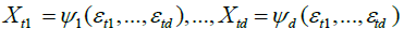
Let  be a d-variate linear process independent of the form:
 (1)
(1)
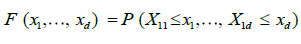
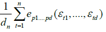
Given the set of observations (X11,..., X1n),...,(Xn1,..., Xnn), let 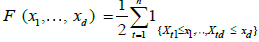 be the empirical marginal distribution function, where 1A denotes the indication function of set A; we can then introduce the multivariate empirical process for
  , a normalizing factor to be discussed later.
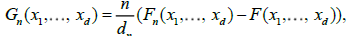
The asymptotics for Gn(x1,...,xd) when the observables are independent and identically distributed (i.i.d.) or weakly dependent has long been well understood by Dudley [1] for a review. In this paper, we shall focus instead on the case where Xt is a long memory process, in a sense to be rigorously defined in section 2, Marinucci [2] developed in the bivariate case. Our work can hence be seen as an extension to the multivariate case of bivariate results from Marinucci [2]; see also Arcones [3] for results in the multivariate Gaussian case.
The structure of this paper is as follow. In section 2, we introduce our main assumptions and we discuss Hilbert space techniques for the analysis of multivariate long memory processes. Section 3 presents first a convergence result for the finite dimensional distributions of  the limiting elds can be viewed as straightforward extensions of the Hermite processes considered by Dobrushin and Major [4], Taqqu [5] and many subsequent authors. We then go on to establish a multivariate uniform reduction principale, which extends Dehling and Taqqu [6] and is instrumental for the main result of the paper, i.e. a functional central limit theorem for proofs of intermediary results are collected in the appendix.
Our first condition relates to some unobservable sequences εt1,...,εtd, which we shall use as building blocks for the processes of interest.
Condition A. The sequences {εt, t = 1,...} are jointly both Gaussian and independent, with zero mean, unit variance and auto covariance functions satisfying, for 
 (1)
(1)
Condition A.
It is a characterization of regular long memory behaviour, entailing that εt have non-summable autocovariance functions and a spectral density with a singularity at frequency zero (see for instance, Leipus and Viano [7] for a more general characterization of long memory). Here, ∼ denotes that the ratio between the right and left-hand sides tends to one, and  are positive slowly varying functions [8].
 , for all c > 0 and La (.) is integrable on every nite interval.
The observable sequences  are subordinated to εt in the following sense.
Condition B.
For some real, measurable deterministic functions
We stress that we are imposing no restriction other than measurability on  for i = 1,...,d, and consequently condition B covers a very broad range of marginal distributions on Xt; in particular, although Xt are strictly stationary they need not have nite variances and hence be wide sense stationary. If we denote by
  , the cumulative distribution function of a standard Gaussian variate. As in many previous contributions, our idea in this paper is to expand the multivariate empirical process into orthogonal components, such that only a nite number of them will be non-negligible asymptotically. Our presentation will follow the notation by Marinucci. Denote by Hp(.) the p-th order Hermite polynomial, the first few being,
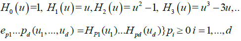
It is known that these functions form a complete orthogonal system in the Hilbert space  denoting a standard Gaussian density. Also, for zero-mean, unit variance variables
  with Gaussian joint distribution we have,
 for
for  and 0 if not.
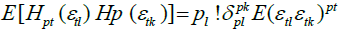
Hence, under condition A,
where
In view of (1) and (2), and using the same argument as in Taqqu [9], theorem 3.1, and Marinucci [2]; here
We can expand  into orthogonal components, as follows:
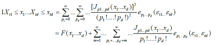 (3)
(3)
where the coefficients  are obtained by the standard projection formula

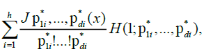
From (3) we have, for any fixed  ,
,
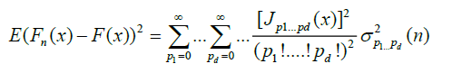 (4)
(4)
It is thus intuitive that the stochastic order of magnitude of  is determined by the lowest
  terms corresponding to non-zero such that,

In the sequel, it should be kept in mind that the cardinality of  (which we denoted h) can be larger than unity, i.e. the minimum of
  can be non-unique; of course,

Condition C.
Condition C entails that the covariances of  are not summable, i.e. they display long memory behaviour.
Note that for condition C to hold it is not necessary that the observables X1,...,Xd are long memory; the autocovariances of one of them can be summable.
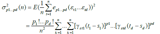
Now let,

be the square root of the asymptotic variance of 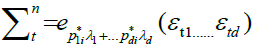 , we need the following technical condition.
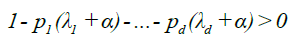
Condition D.
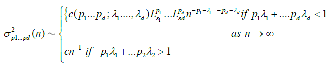
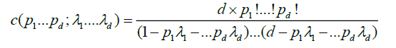
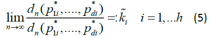
As  exists and it is non-zero, i.e. there exist some positive, finite constants
  such that
Of course, we have
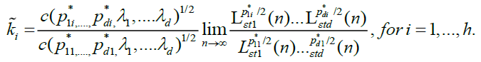
Thus, condition D is a mild regularity assumption on the slowly varying functions  .
.
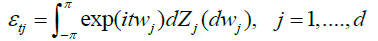
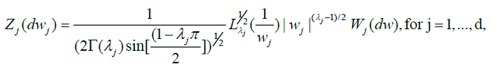
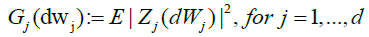
Define the random processes
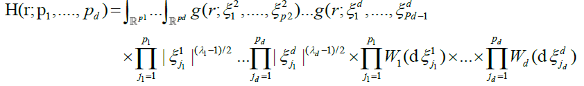
where W1(.)...Wd(.) are independent copies of a Gaussian white noise measure on  , the integrals exclude the hyper diagonals, and
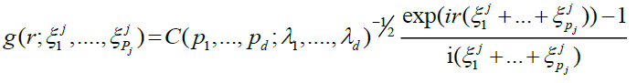 (6)
(6)
for j = 1,...,d.
Indeed, the following result is a direct extension of results by Marinucci [2]
Proposition 1
Under conditions A, B, C and D, 
 (7)
(7)
where  denotes weak convergence in the Skorohod space
  . We provide now a uniform reduction principle for the multivariate case.
Proposition 2
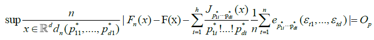
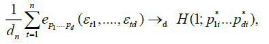
Under conditions A, B, C and D,
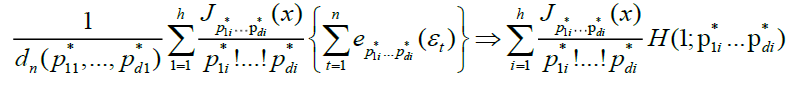
Theorem
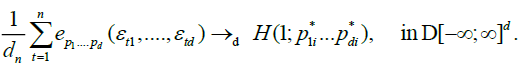
Under conditions A, B, C and D,
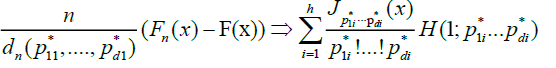
where denotes weak convergence in the Skorohod space .
.
Proof of Proposition 1
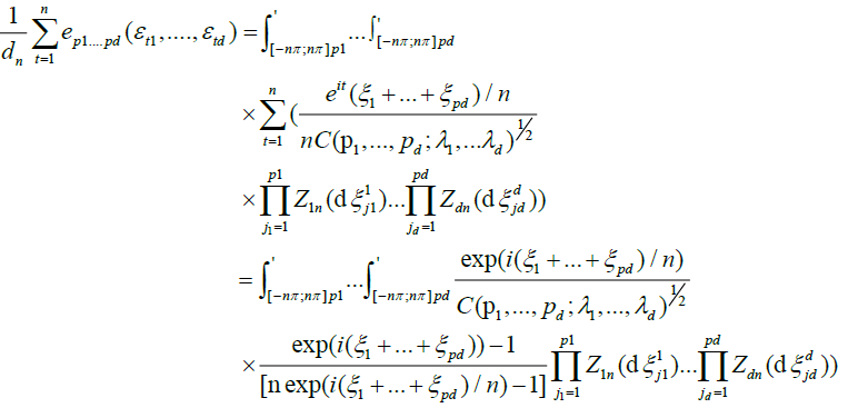
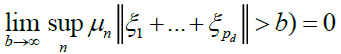
In the sequel, we concentrate, for notational simplicity, on the case h = 1 and we write for brevity 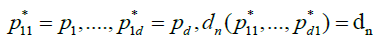 when no confusion is possible. We focus first on the asymptotic behavior of
 (8)
(8)
Here our proof is basically the same as the well-known argument by Dobrushin and Major [4] for univariate Hermite polynomials, and Marrinucci [2] for bivariate case, we omit many details. The sequences εtj can be given a spectral representation as
Where, by condition A and Zygmund’s lemma [10]
With governing spectral measures:
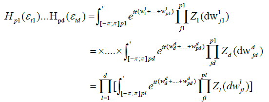
Hence, by the well-known formula relating Hermite polynomials to Wiener-Ito integrals [11]
Next we de ne new random measures on the Borel sets  by
by
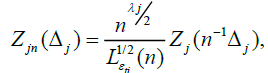
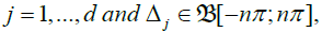 so that after the change of variables
  for
for  equation (8) becomes:
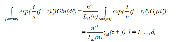
Now consider the spectral measures,
 and a piecewise constant modification of the Fourier transform, i.e.
Where  the last step follows from
The following result is a simple extension of lemma 1 in DM [4] and lemma A.1 in Marrinucci [2].
Lemma 1.A
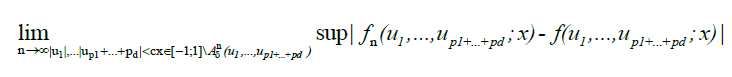
As we have, uniformly in every bounded region

Where
Proof
Let

it can be verified that
Now define the set

As in DM [4], by the standard properties of slowly varying functions, it can be shown that, for any c,
Where

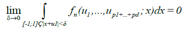
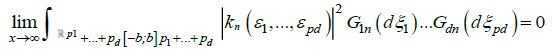
To complete the proof, we just need to show that,
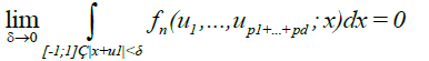 (9)
(9)
 (10)
(10)
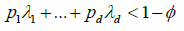
For every l = 1,..., p1 + ... + pd, such that |ul| < c. We assume without loss of generality that p1,...,pd# 0, otherwise we are back to the univariate case.
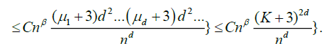
Choose a positive ![]() small enough that
small enough that
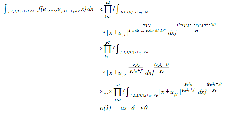
Then
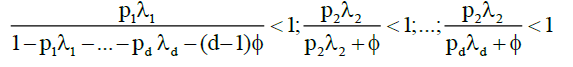
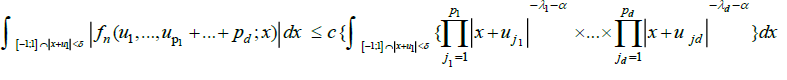
Hence by Holder inequality we obtain for equation (10) that
For (9), we can argue exactly as in DM [4], equations (3.9) - (3.10), to show that there must exist α > 0, small enough that
and such that

Then, again as in DM (1979), equation (3.11),we obtain
whence the proof can be completed by the same argument as for (10).
Lemma 2. A
Let Gjn be sequences of non-atomic spectral measures on B on tending locally weakly to d non-atomic spectral measures Gj0, j = 1,…, d, Kn(ε1,… εpd) a sequence of measurable functions on  tending to a continuous function
 in any rectangle
  Let the
 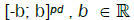 functions Kn(.) satisfy the relation
 (11)
(11)
uniformly for n = 0, 1….Then the Dobrushin-Wiener-Ito integral
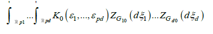
exists, and as 

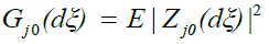
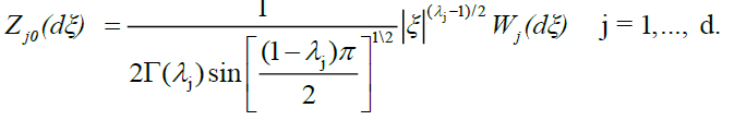
where ZGj0(.) denotes a random to be dened below, and based on Gj0(.), j=1,… d
Proof
The proof is identical to the argument by DM (1979, p.41); the définition of local weak convergence is given on page 31. Note that here we have d different random measures, ZG1n(.) ... ZGdn(.); as these d measures are independent, however, the extension to product spaces is straight foward.
To establish the asymptotic behaviour of (8), we apply Lemma 2.A with the choice.
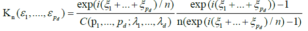
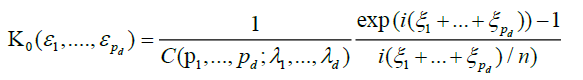
and
The convergence of Kn (.) to K (.) in any rectangle 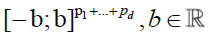 is immediate.
The convergence of the measures Gjn (.) to Gj0 (.), j = 1,..., d is proved in Proposition 1 by DM [4]. The crucial step is then to show that equation (11) holds.
Consider the d measures

and

Note that  is the Fourier transform of
 and
and  is the Fourier transform of
 ![]() . By lemma 1.A,converges to
. By lemma 1.A,converges to  uniformly in every bounded region, and hence by lemma 2 in DM [4] we have that tends weakly to the measure
 ![]() ,which must be finite. Moreover, weak convergence entails that
,which must be finite. Moreover, weak convergence entails that
(Condition (1.14) in DM [4]), and in turn this implies (11). We have thus shown that, as
 (12)
(12)
And also, if we view the left-and right-hand sides of (12) as constant random functions from 
 (13)
(13)
Now note that, for any 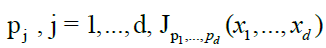 belongs to
  by its own definition; proposition 1 then follows from the functional versionof Slutsky's lemma and the continuous mapping theorem, see for instance Van Der Vaart and Wellner [12], section 1.4.
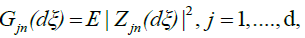
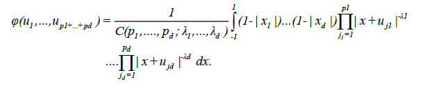
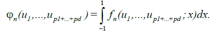
Now introduce the function

For the arguments in the sequel, we use the following notation. Let aj ; bj be any uplet of real numbers  we can define the blocks

It is obvious that, if x1i,...,xdl, for i = 1 ,....,I, and l = 1i,....,L, are no decreasing sequences, then the sets  are all disjoint. Given any multivariate function
  we can hence define an associated (signed) measure by,
The resulting measure can be random, for instance if we take T (;...; ..) = Sn (.;...; .) as we shall often do in the sequel. The following result provides an extension of lemma 3.1 in Dehling and Taqqu [6] to the random measure case.
Lemma 3.A
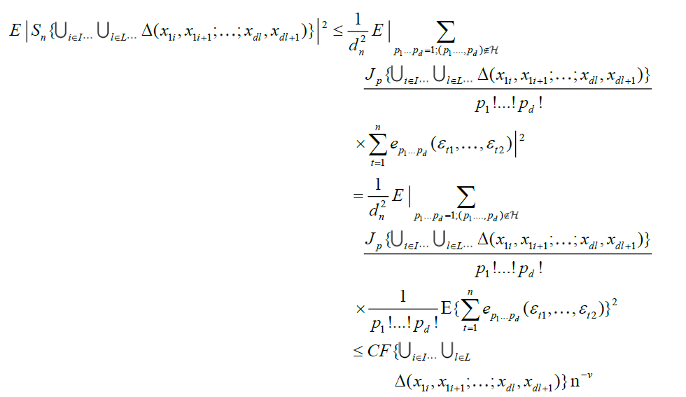
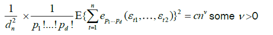
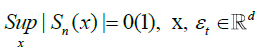
Under conditions A, B, C and D, there exist some ν > 0 such that, as
 (14)
(14)
Proof
With p1...pd = p, in view of equation (3), we obtain
because
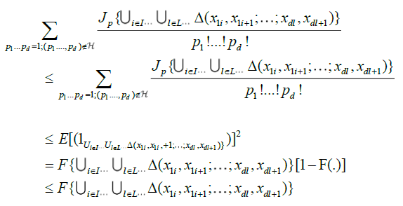
for all (p1...pd) such that 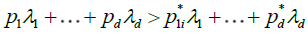 .
.
For notational simplicity and without loss of generality, we consider only the case h = 1; also, we write  for
for  . We use a chaining argument which follows closely the well-known proof of Dehling and Taqqu [6].
Set
and

it can be readily verified that, for any give block 
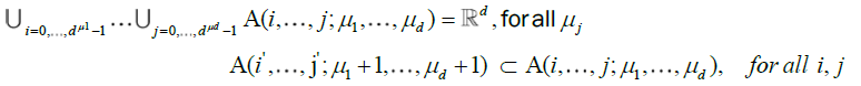
The idea is to build a "fundamental" partition of  Rd, such that
 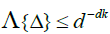 , for each Δ in this class and for a fixed
  . Starting from this fundamental class, we will then dene coarser partitions by summing blocks made up with
 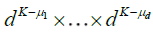 fundamental elements, μj = 1,2,...,K for j = 1,...,d. The latter blocks will then be used in a chaining argument to establish an uniform approximation of Sn(x1....,xd). More precisely, put


The sequences 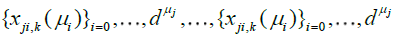 become finer and finer as μj and j = 1,...,d grow, i.e.

 .
.
Clearly, we have
For the following, we put i = jiand j = jd.
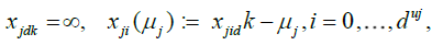
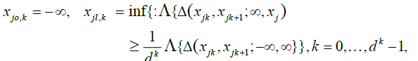
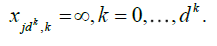
Now consider the sets
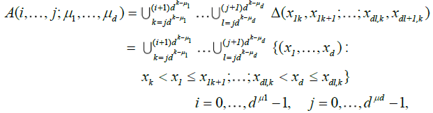
which define a net of refining partitions of ![]() , i.e.
, i.e.
Note also that
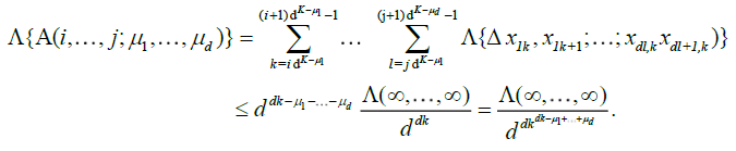
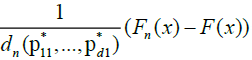
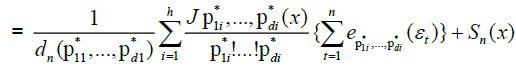
Define 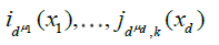 by
by

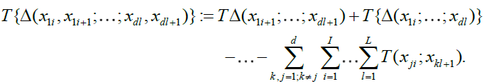
And in Marinucci [2], we can use the decomposition
 (15)
(15)
 (16)
(16)

 (17)
(17)
 (18)
(18)
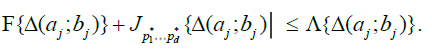
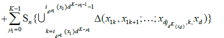
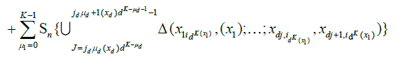
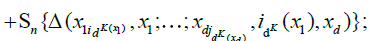
in words, we have partitioned the random measure Sn(x1,...,xd) over 2d sets of blocks: those were the corners are all smaller than x1,...,xd (15), those where the corners have coordinate x2,...,xd−1 and the top corners have coordinate xd (16), those where the right corners have coordinate others variables x1,...,xd−1 (17), and a single block which has (x1,...,xd) as its top right corner (18). Now
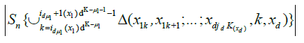
Therefore,
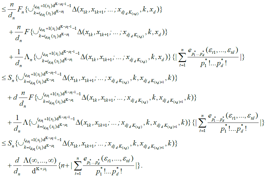
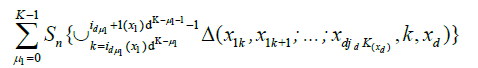
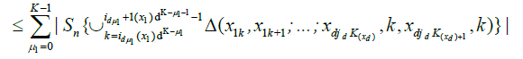
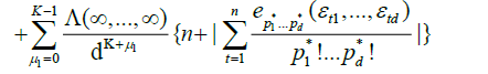
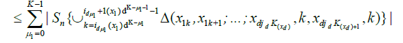
By an identical argument in Marinucci (2005), finally, we have

Since for any 
we have


 .
.
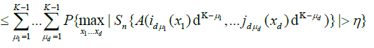
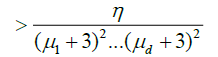
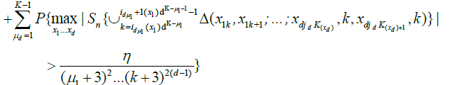
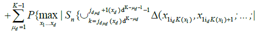
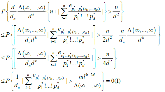
Now note that, by lemma 3.A and Chebyshev's inequality,
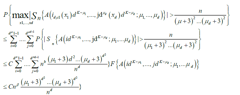
And hence
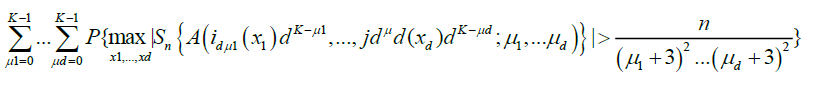
 (19)
(19)
Equation (19) is immediately seen to be o (1). Also, in Marinucci [2], we obtain
The remaining part of the argument is entirely an analogous
 .
.
 .
.
From the prepositions 1and 2, we have, as n to infinity
 and thus the result is established.