International Journal of Advanced Research in Electrical, Electronics and Instrumentation Engineering
ISSN ONLINE(2278-8875) PRINT (2320-3765)
ISSN ONLINE(2278-8875) PRINT (2320-3765)
Chandrpal singh1, Abhaskumar singh1,Priyeshkumar pandey2,Harmendra Singh2
|
| Related article at Pubmed, Scholar Google |
Visit for more related articles at International Journal of Advanced Research in Electrical, Electronics and Instrumentation Engineering
The Power Donut is a state of the art instrumentation platform designed for data acquisition and data logging applications on high voltage, overhead conductor systems. The Power Donut2 is completely self-contained. it is self-powered, it measures current ,voltage, MW, MVars, MWh ,conductor temperatures, stores data on board, and it transmits data on demand using a radio modem. The integration of a power line sensor network (PLSN) has been proposed to monitor such a utility asset’s status for maximizing existing power grid utilization with minimal risk of degradation and for extending the lifetime of said assets. The included sensors and wireless data communications system allow for the transmission of data pertinent to determining the ampacity of assets. Six USi Power Donut devices were used on 220 Kv transmission lines of a utility partner.The technology used inside the "donut" is a Motorola G24 cellular telephone module. The G24 unit is installed in the "Power Supply" pocket. The G24 product provides “2.5 G” service.
Keywords |
| Conductor Temperature, Dynamic Thermal Rating (DLR) of line, line sag and tension monitor, transmission line troubleshooting, alarm monitoring. |
I.INTRODUCTION |
| Over the past two decades power usage has significantly increased with little corresponding development of the power grid infrastructure. As a result, fears of overloading existing power lines have emerged. Overloading occurs when the line is heated to a temperature at which the conductor begins to degrade, causing, among other issues, irreparable sagging in the lines .The Power Donut presents a solution to this problem .It contains sensors which measure the line current, voltage and temperature along with transceivers which allow it to transmit its data via cellular towers and the internet to centralized servers for data processing. Combined with nearby weather conditions, such as wind speed, wind direction, ambient temperature, air pressure, and relative humidity, accurate predictions can be made concerning the line temperature and ampacity for a period of time following the calculations. The collected data enables the determination of both the steady state and dynamic thermal ratings of a given power line. In this paper we discussed about the working of power donuts or we can say that thermal line monitoring of transmission. Also discussed about sag and tension of transmission line. |
II.DYNAMIC LINE RATING |
| Dynamic line rating determination methods are generally divided in direct and indirect methods. It depends on the source where the line between direct and indirect methods is drawn: some consider only the sag determination methods as direct methods, whereas most consider all the methods monitoring the transmission line characteristics as direct methods. The IEEE 738 method employs an empirical estimate to obtain the Convection Heat Flow “qc” as in the heat flow equation displayed below. Where m is the mass per unit length of the transmission line, Cp is the specific heat of the line, Tc is the conductor temperature, qc is the rate of heat loss due to convection cooling, qr is the rate of heat loss due to radiation cooling, qsis the rate of heat gain due to solar heating, I is the line current, and R (Tc) is the line resistance per unit length at the specified line temperature. |
| Standardard heat flow equation |
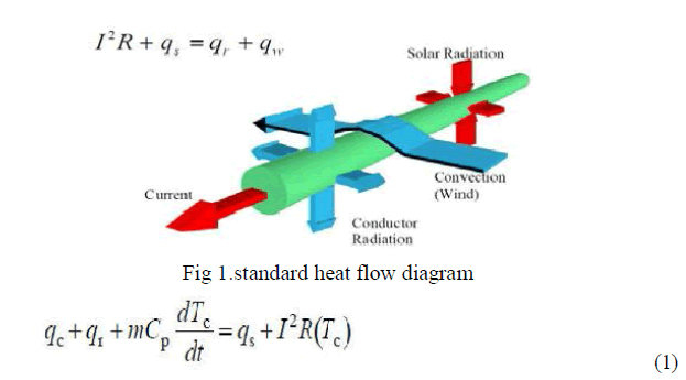 |
| This equation is used to predict the duration a line can be held at a given load without overheating and is used in the generation of the I-T characteristic curves presented later in this document. |
| qc = qs + I2Rac(Tc)– qr - mCpdTc/dt(2) |
| Rearranging the standard heat flow equation, the convection heat flow “qc” can be calculated using parameters obtained from field measurements: |
| Racis computed using the conductor specifications, the conductor temperature and the ambient air temperature |
| ambient air temperature Tamb- can be measured using a weather sensor conductor temperature |
| conductor temperature Tc- can be measured using a Power donut |
| current I in conductor - can be measured using a Power donut |
| m and Cpare obtained from conductor data sheets |
| qsand qrare calculated using the proven algorithms from actual field measurements |
| dTc/dtis calculated using the rate of change of Tcwith time |
 |
| Where, |
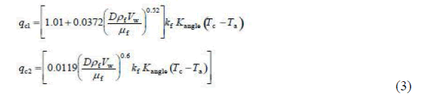
| qC1is applies for low winds but incorrect for high wind speeds. |
| qc2is applies for high winds but incorrect for low wind speeds. |
| In steady-state, the derivate term in the heat balance equation (1) becomes zero, resulting in equation (3) that can be used to determine line ampacity: |
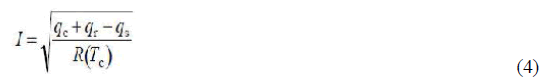 |
| Equation (4) above represents the current that would result in a steady-state temperature at the specified input Tc and at theprovided input atmospheric conditions. By substituting the maximum allowable line temperature for Tc, one candetermine the line ampacity. |
III. INSTALLATION |
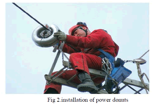
| The Power Donut2 needs no supporting infrastructure. It attaches to the conductor by means of a hot stick and can be installed without taking an outage. Bushing assemblies match the Donut hub to the customer’s conductor and are available for the entire range of transmission conductor sizes including bundled conductor configurations. The Donut is powered by magnetic flux coupling from the conductor and operates on all voltage level systems up to 500 kV. |
 |
IV.POWER DONUT SERVER SOFTWARE FUNCTION DESCRIPTION |
| The Power Donut uses GSM/GPRS/Edge wireless data service to communicate with the customers' data concentrator/server. The technology used inside the "donut" is a Motorola G24 cellular telephone module. The G24 unit is installed in the "Power Supply" pocket. The G24 product provides “2.5 G” service |
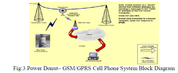 |
| The Power Donut2’s built-in frequency hopping spread spectrum radio is capable of transmitting data at up to 115 kbps and a distance of up to five miles. The Donut™ maybe used in real time, Wide Area Management Systems, in SCADA and Energy Management Systems, and has on board flash memory for analog and event data logging. Users retrieve data from the Donut™ using the USi Ground Station2. Ground Stations can also be made portable for mounting in a van or helicopter |
V.IMPLIMENTATION |
| Six PD were installed at different locations of a 220 kV transmission network, and data from May to July of 2010 was collected at a 1 minute sampling period. This data included line current (I), line-to-neutral voltage, power and reactive power, conductor temperatures (Tc), and line inclination. This data was augmented with environmental data from local weather stations, which included wind speed average and direction, air pressure and temperature, relative humidity, and rain accumulation. Other data required by the IEEE 738Standard equations, such as the line latitudes, longitudes,elevations, and resistances at low and high temperatures were collected along with the corresponding absorptivity and emissivity. Using the collected data, the steady-state ampacity of each line was calculated for every minute, using equation (4). These discrete ampacities are shown for a period of time in Fig. 1, along with the line current, average ampacity over the given period, and the current rating that is currently in use for the line. The ampacity plot merely shows the maximum allowable current that would result in a steady-state temperature which would not degrade the line. Note that the steady state temperatures would be reached at a later time, depending on the system time constant. As seen, due to the dynamic nature of the environmental variables, the ampacity varies significantly even though the line current is much less variant. |
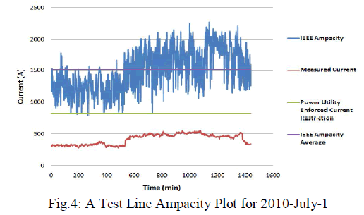 |
| In Fig. 4, the IEEE Ampacity curve represents the instantaneous steady-state ampacity of the line at each minute. The Current line represents the actual load on the wire on July1st. The employed current restriction curve represents the maximum current currently allowed on the line at a given time, also denoted as the maximum allowable conductor current for a long-term emergency situation (SLTE) in the corresponding data files. The IEEE ampacity average line represents the average of the calculated IEEE ampacity data for July 1st .The IEEE calculated ampacity curve actually represents conservative limit, since the current on the line must be held at that ampacity limit for longer than 20 minutes before the lineTemperature approaches its safe operating limit. As such the limit currently enforced is even more conservative. Analyzing these plots may be useful, however, in determining new conservative maximum safe operating currents. Of note is the large variability calculated in the ampacity values. As can be seen in Fig. 4, the IEEEcalculated ampacity varies greatly over the selected period. For this dataset the maximum change in ampacity was almost 900A/min at about 3:00PM with an average change of about 115 A/min |
| Fig.5 shows how much the environmental conditions vary over the same period. |
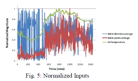 |
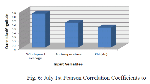
| Just looking at the two graphs, one can see how the ampacityResults from Fig. 4 mirror the variability presented by wind speed and direction and the general curvature of air temperature in Fig. 5. To verify the impact each weather condition had on the resulting ampacity, a Pearson Correlation Coefficient Matrix was produced for July 1st. The results are provided in Fig. 8. The Pearson Correlations presented in Fig. 8 confirm the impact the selected variables had on the ampacity, suggesting high correlation, in the order of importance, to wind speed, air temperature, and the angle between the line and wind azimuths. |
 |
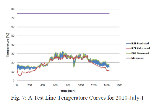 |
| The Non-Steady-State Heat Balance equation provides more useful results, allowing an operator to determine the effects increasing the load on a line will have on its temperature, and the amount of time a line could be held at that load before risking its integrity. Fig. 7 and Fig. 8 compare the IEEE calculated line temperatures based on transient equation 2: |
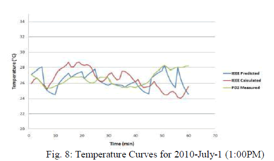 |
| In Fig. 7 and Fig. 8, the PD2 Measured curve is the actual conductor temperature as measured by the Power Donut. We used two different methods in implementing the transient conductor temperature, referred to as the “IEEE Calculated” curve and the “IEEE Predicted” curve. The “IEEE Calculated” curve was generated by using the initial conductor temperature measured by the power donut. The differential equation 1 uses all remaining variables at every minute to determine the change in conductor temperature and, thus, all following conductor temperatures for the remainder of the curve (note that achieving similar results would require accurate weather predictions for the period of data generation). The “Maximum” line, appearing only on Fig. 7, represents the maximum allowable conductor temperature (SLTE) as provided by our power utility collaborators. As shown in Fig. 7, the “IEEE Predicted” curve tends to be closer to the measured conductor temperature, because it involves resampling the measured temperature every five minutes, before predicting the temperature for the following period. As shown in Fig. 7, the “IEEE Calculated” curve shows a more significant deviation from the actual temperature .Using data sampled by the PD or averages of said data, predictions can be made concerning the conductor temperature for short periods of time with dependable accuracy. Due to the complexities and nonlinearities of the differential equation, this process is performed using a simple “for” loop, which recalculates the temperature differential for every minute, using solar heat gain rates recalculated for the new instance in time. An example of the calculated results is provided below: |
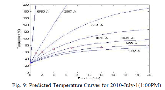 |
| Fig.9 presents samples of the temperature curves predicted at1:00PM on July 1, 2010 given step changes in current to the displayed values. The horizontal bar at 75°C identifies the thermal capacity of the line. Due to implementation of the simple “for” loop approach, the resulting durations are limitedto minute-wise accuracy, which is sufficient for our application and actually assists in providing more conservative results. The results above are reorganized into I-T characteristic curve plots to provide the data in a more easily interpretable form. As such, an operator can see at a glance the highest current that can be placed on a line for a given duration. |
VI.CONCLUSIONS |
| The data collected by the power donut and transmitted from nearby weather stations allows for accurate predictions to be formed using the equations presented in the IEEE 738 Standard. With these predictions, asset utilization can be optimized with confidence, posing minimal risk to the integrity of power grid assets. DLR is truly Smart Grid technology and it is very possible that DLR will become more commonly used, or even required technology. For DLR implementation, the analysis of DLR profitability and potential could be evaluated based on statistical and probabilistic analysis of offline DLR measurements. The DLR implementation ought to proceed from probabilistic design to deterministic operation. Using these predictions, operators can make informed decisions on diversion of power in times of crisis, shifting loads to protect existing power grid infrastructure, while still meeting ever-growing demands. Experimental results demonstrate the potential impact of these devices in terms of better grid utilization and improvement in system reliability |
References |
|