Walid Y Alali1 and Haider Alali2*
1Department of Economics, University of Oxford, Oxford OX1 3UQ, United Kingdom
2Department of Economics, Oxford Institute for Economic Studies, Oxford OX1 3AE, United Kingdom
Received: 28-Jun-2023, Manuscript No. JSS-23-104113; Editor assigned: 30-Jun-2023, Pre QC No. JSS-23-104113 (PQ); Reviewed: 14-Jul-2023, QC No. JSS-23-104113; Revised: 27-Dec-2023, Manuscript No. JSS-23-104113 (R); Published: 04-Jan-2024, DOI: 10.4172/JSS.10.1.003
Citation: Alali H, et al. Production and Foreign Investment Affected by Brexit. RRJ Soc Sci. 2024;10:003.
Copyright: © 2024 Alali H, et al. This is an open-access article distributed under the terms of the Creative Commons Attribution License, which permits unrestricted use, distribution and reproduction in any medium, provided the original author and source are credited.
Visit for more related articles at Research & Reviews: Journal of Social Sciences
We resolve several scenarios of post-Brexit using a multi-country simulations model of neoclassical growth. We started by assuming the UK unilaterally imposed much tighter restrictions on foreign direct investment and trade with other EU countries. Then we assume the European union imposes and retaliates against the United Kingdom's same restrictions. In the final scenario, the UK has reduced restrictions on other countries through the post-Brexit transition period. The model predictions depend mainly on the policy response to MNCs investments in technology capital, knowledge accumulated from investments in brands, R and D and organisations used concurrently in their foreign and domestic operations.
Brexit; Economic growth; Investment; FDI; Trade policy; International trade; Economic integration; Multinational firms; Management of technological innovation and R and D
JEL-Classification: C32; E65; F13, F15; G32
The vote to leave in the Brexit referendum on 23 June 2016, means that trade costs will rise and that UK and EU multinationals will no longer have free movement of capital across each other's borders, as their subsidiaries will be subject to more regulations. Rigour and higher production costs, as restrictive policies evidence, Kalinova, Palermo, and Thomsen, who discuss indicators of the OECD investment division that measure the restriction of foreign direct investment in member countries, specifically regulatory restrictions such as foreign equity limits, screening and approval, and personnel restrictions[1]. The two principals, the operational regulations. And invested in the European union before the referendum. To perform our analysis by extending the model of multi-country dynamic general equilibrium of McGrattan and Prescott which introduces trade frictions and allows for bilateral costs in FDI, which then allow us to examine the partial solution of an economic union[2]. The key feature of the framework is technology capital, which is the experience accumulated from brands, investments in R and D and organizations that multinational companies can use simultaneously in their domestic and foreign operations. This capital plays an essential role in FDI, as multinational companies have more locations to use as countries become more open. In our environment, a country that erects barriers to inward FDI suffers welfare losses because foreign innovation is effectively hindered and costly domestic investment in technology capital is required to replace foreign investment. Increase the technological capital of the country that is becoming more closed in the countries with benefits that remain open as the capital can be used simultaneously in foreign subsidiaries. If two countries (or unions) simultaneously erect barriers to each other's foreign direct investment, the balancing forces that is, preventing innovation and increasing domestic investment will have consequences that are hard to predict without a framework like ours, especially given that other countries will respond to this policy. Changes in the global general equilibrium situation. If the costs of imported goods increase simultaneously, the losses will be greater because consumers want the foreign items, but producers cannot shift costless to producing domestically and shipping the goods.
In the Brexit baseline scenario, we assume that the United Kingdom and the remaining countries of the European Union impose tighter restrictions on both foreign direct investment and trade with each other. To provide an intuition for these results, we first analyse each policy change independently. To analyse the impact of changes in FDI policy, we first assume that the UK tightens EU capital unilaterally, and then assume that both economies restrict the movement of capital across each other's borders. If the UK acts alone and tightens restrictions on foreign direct investment in the EU, EU companies have less incentive to invest in technology capital. Lower investment by EU firms negatively affects the UK. With less technology capital coming from abroad, British companies must invest more in research and development and other intangible assets, which is costly. The next step is to consider the effect of higher trade costs alone, assuming no change in FDI policy. We start by assuming a unilateral move by the UK to restrict EU goods and then EU countries retaliate. As trade costs rise, multinationals shift from less exporting to FDI, but the effects on the innovation of the multinational parents are much less than in cases with higher FDI costs. We are experimenting further where there are higher costs of trade and investment between the UK and the EU but lower costs of FDI flows into the UK than other countries. We include these experiments to compare the welfare of UK citizens in the base scenario with the alternative scenario in which the UK negotiated new trade and investment deals with non-European countries.
To make quantitative predictions, we parameterize the model using data across countries in the run up to the Brexit referendum. Parameters are chosen to ensure that population, corporate tax rates, real GDP, bilateral foreign direct investment flows, and bilateral trade flows are the same in the model and data. In the base scenario, we assume that trade costs and FDI costs rise by 5% points, starting in 2019 and fully in by 2022. In the case of FDI costs, this cost increase is equivalent to a 5% reduction in total production. As negotiations are ongoing and there is uncertainty about the specific policies that will be enacted, we are also experimenting with the timing and size of cost increases. Since we are working with a dynamic model, we can compare predictions of immediate referendum responses to long term outcomes. Given that the accumulation or nullification of technology capital plays a central role in the model, the long run in our model is approximately 50 years after the referendum. Moreover, between the referendum and the implementation of the actual policy, firms and households benefit from existing capital inputs that can be used in production before current account flow costs rise. Thus, the UK and EU economies could emerge unexpectedly strong despite Brexit.
In the base scenario, with the UK and the EU raising both trade costs and FDI mutually by 5% points, we find welfare losses of 1.4% and 2.3% for UK and EU citizens, respectively. If we just raise the costs of trade, with no restrictions on foreign direct investment, the losses would be much lower, around 0.2% and 0.02% for UK and EU nationals, respectively. The main reason for the difference is that higher trade costs lead consumers to substitute between UK and EU varieties and producers to substitute between exports and FDI, but they have little effect on innovation by multinational parents. Innovation drives investment in technology capital, which depends critically on the relative degrees of countries' openness to foreign direct investment. If the UK acts alone and tightens restrictions on FDI in the EU, EU companies have less incentive to invest in tech capital and reduce their investment by an average of about 5% in the first decade and by more than 6% in the long term, regardless. of changes in trade policy. As technology capital is used in all locations around the world, the impact on production and welfare is significant. If the EU retaliates and lifts restrictions on FDI in the UK, we would find a significant decrease in technology capital investment in the UK ultimately by 30% in the base scenario and a 12% increase in technology capital investment in the EU. Since the EU is much larger in terms of population and production capacity than the UK, UK companies have more subsidiaries affected by the policy change and therefore have less incentive to invest. This turns out to be important to the EU's well-being because the UK was a big investor in the pre-Brexit period.
If the UK reduces trade and FDI costs to other countries, we find welfare gains rather than losses. We first look at cutting costs in the US and Canada by 5% points on both trade and foreign direct investment. In this case, we would expect a welfare gain for the UK of 0.7%, well above the 1.4% loss in the baseline, with little change for the EU. The UK is effectively replacing a lower TFP trading and investment partner with a higher TFP partner. If the UK cuts costs on all non-EU partners, again by 5% points, the UK welfare gain is 1.3%. In both scenarios, lowering the costs of FDI is key to increasing welfare because innovation increases exponentially in other areas. All countries except the European Union win.
Most of the relevant work estimating the effect of Brexit on current account flows has been empirical, based either on the synthetic facts method or on gravity regressions. Campos and Coricelli use a synthetic counter facts method, comparing actual FDI inflows into the UK to those of a synthetic UK whose data is a weighted sum of data from control countries in this case, the US, Canada and New Zealand that did not enter European Union[3]. They estimate that inflows would fall by 25% to 30% if the UK did not join the union. See Campos, Coricelli, and Moretti for details of the method and results for all EU members[4]. See Barrell and Pain and Pain and Young[6] for other work to estimate the effect of EU membership on FDI flows and macroeconomic groups[5,6]. Dhingra, et al., summarize recent work analyzing the overall effect of EU membership on FDI stocks and flows[7]. Most relevant to our paper is the work of Bruno, et al., which estimates gravity regression with bilateral FDI flows in 34 OECD countries as a dependent variable and uses source and host country characteristics, including EU membership, as independent variables[8]. Bruno, et al., found that EU membership has a positive effect an average of 28% across regression profiles on FDI inflows. In contrast to this, Bruno et al., predicted that leaving the union would result in a decrease of 22% (or 0.28/1.28), which is close to the estimates of Campos and Coricelli[9]. In the base scenario, our model predicts that inward FDI in the UK will rise, not fall, because other countries increase investment and outward FDI in response to Brexit policies.
Other related work uses quantitative theory to estimate the impact of Brexit. Steinberg analyzes the impact of higher post-Brexit trade costs in a dynamic model and estimates that UK production will be lower in the long run [10]. It forecasts a decline in output of 0.4% to 1.1% below pre-Brexit levels. In our baseline simulations with the UK and EU both raising costs on trade and FDI to each other, we found larger effects, with output falling by about 1% compared to the trend in the first decade of the transition, and eventually falling by an even larger amount. from 3%. Arkolakis, et al.,[11] which analyzes a static economy with costs on both trade and FDI, find larger effects of increasing costs on FDI than on trade, which is consistent with our findings. In recent work, Anderson, Larch, and Yotov[12] used a dynamic model in the spirit of McGrattan and Prescott studies the interaction between foreign direct investment and trade but does not analyze Brexit.
However, the mechanism underlying our findings, which critically depends on how Brexit affects global investments in technology capital, differs from that of Arkolakis, et al.,[11] which depicts innovation as the creation of differentiated goods in single product firms, with labour being the sole factor of production. See also Antras and Yeaple[13] for a survey of theories of multinational corporations in international trade. Contrary to ours, the theories they review assume that capital is immobile across countries and is therefore not suitable for analyzing FDI flows. Moreover, our analysis is relevant to macroeconomics, while Arkolakis, et al.,[11] Manufacturing sector analysis only.
In the first section, we describe the model, and in the second, we discuss how the model parameters were determined using pre-Brexit data from national and international accounts. In the third section, we report the results of the Brexit simulations, and in the fourth section, we check the sensitivity of the main results. The fifth section concludes.
Model
There are I economic unions, which are groups of countries, states, or provinces that place little or no restrictions on cross border shipments or direct investments of multinational corporations. Each economic union is distinguished by its production capacity, TFP, its policy that governs traded goods, and its policy that governs foreign investments, and these characteristics are taken from multinational companies when making their decisions related to production and foreign investment. The multinational corporations in each consortium invest in technology capital, which can be used for production at home or abroad. If produced at home, companies bear trade costs when shipping goods to foreign customers. If they are produced abroad, subsidiaries of these companies face organizational costs and production costs. More specifically, for each economic union i at a time t the total number of sites, Nit, where domestic or foreign firms can operate and the TFP level, Ait. Foreign multinationals are associated with our proprietary technology, which we index by ω, and their production decisions are based on trade costs for shipments to Union i, denoted by ζit(ω), and Union i′s degree of openness to the firm's investment, denoted by σit(ω), another explanation for the σit(ω), parameters are that they are not policy parameters but represent differences in union characteristics, such as language, that inhibit foreign investment. See, for example, Keller W Yeaple [14] and Ramondo [15]. These differences could influence pre-Brexit levels of openness, but not the post-Brexit transition. In this section, we describe the technologies available to these companies and the preferences of the families representing shareholders.
Firm Problem
Following McGrattan and Prescott[2], we start by describing technologies for domestic and foreign factories and then derive aggregate production functions at the firm level and the level of the economy as a whole. Considering these aggregate production functions, we can identify the main problem of a multinational company that is maximizing profits all over the world.
A company with (ω), technology selects labour and capital in all locations around the world. Some capital is tangible (such as structures and equipment), and some are intangible (such as research and development, brands, and organizations). Some intangible capital is site-specific (for example, lists of local clients or clients), and some are non-competitive and can be used in all locations (for example, research and development). To simplify the presentation, suppose that the capital and labour inputs for the site can be combined into a composite input(z). Suppose also that the firm has invested in research and development and has a "blueprint" that when combined with other inputs results in z
y=AiZ1-φ (1)
At one location in i (This does not rule out multiplant firms that deploy more than one blueprint in a location). Assuming that the scheme can be used non-competitively, the firm can use it for production at other locations in i with additional factor inputs. If an economic union is completely open to foreign subsidiaries (established outside the union), then (1) it abstracts technology at the factory level regardless of where the company's parent company is located. If economic union i is not fully open, the output produced in i with technological capital developed abroad, say, in economic union j, is given by
y=σi(ω)AiZ1-φ (2)
with σi(ω) ∈ (0, 1) and ω ∈ Ωj, where Ωj is defined as the set of techniques developed in j. If σi(ω)=1, foreign and domestic firms are treated equally by the government in i, just as in (1). If σi(ω)=0, then i am completely closed to the use of foreign technology ω. It may also be the case that there are greater regulatory costs or restrictions on foreign firms than on domestic firms, without a complete ban on inward FDI, implying a median value of (ω) ∈ (0, 1), subsequently, we analyze aggregate capital flows and estimate the degree of openness for all FDI coming from a country or union, but the analysis can easily be applied to industry wide constraints, such as those that might be warranted by national security concerns.
Since there are diminishing returns to compound inputs z at the plant level, firms increase total output by allocating plant specific inputs proportionately across production sites and plots. Let Nibe the total number of production sites in i. These locations correspond to markets, and markets are a measure of people (in our quantitative work we assume that N i is proportional to population size). Suppose M(ω) is the total stock of technology capital of the firm ω, that is, the total stock of blueprints and other knowledge embodied within the firm. If such a firm operates at i with Zi(ω) units of compound input, it will optimally allocate an equal share of Zi(ω) to the total production potential of M(ω)Ni. In this case, the total output produced by this firm at i will be given by
(ω) = (ω)i{M(ω)Ni}φ Z.(ω)1−φ (3)
Where, again, σi(ω)=1 if ω ∈ Ωi, McGrattan and Prescott[2] derive the aggregate production function, which is the maximum output that can be produced in a country at technology level Ai, a measure of locations Ni, and measures openness (σi(ω)). They show that the function is

Which exhibits constant returns to scaling. Despite this fact, the total output of a group of open economies with σi(ω)>0 is greater than the total output of a group of closed economies. And so, it is as if there are increasing returns when in reality there are no returns.
Here, the composite input (ω) is composed of the site specific labour input, (ω), the tangible capital, KT(ω), and the intangible capital KI,i(ω).
It should be noted that the mathematical calculation underlying production techniques is similar to that found in the standard love of diversity model with constant returns to scale in production, constant elasticity of substitution preferences, and monopolistic competition in the commodity market. In the love of diversity model, setting substitution elasticity between taxa equal to 1/Φ means the same diminishing returns at the plant level as in (1). In all, there are scale effects in both models: gains in openness in the love of diversity model are due to expanding product diversity, whereas our gains are due to expanding the set of sites in which non-competing technological capital can be deployed.
Next, consider the problem of multinational corporations in our environment. They choose factor inputs to maximize the present value of worldwide after tax dividends, which is given by (1−τdt) Σt(ω), where τdt is the stockholders dividend tax rate, pt is the Arrow Debreu rate, and D(ω) is the total dividend payment. Total dividend payments are the sum of payments across economic unions hosting FDI, i.e., Dt(ω)=ΣiDit(ω), where
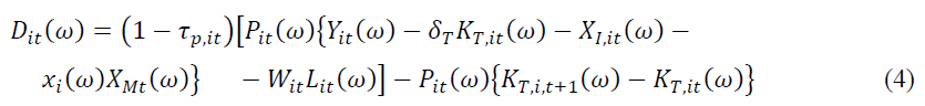
Dividends from economic union i are calculated as after-tax accounting earnings minus retained earnings plus any subsidies for investment in research and development and other intangible assets. The profit tax rate at i is given by τp,i and assessed on taxable income equal to sales Pi(ω)Yi(ω) minus labour payments Li(ω) at the rate Wi, consumption of tangible capital KT,i(ω)t price δT, new investment in intangible capital XI,i(ω) is site-specific, and home investment in new technology capital XM(ω).
Here, we assume that technologies are developed and investments are fully spent in the country where the company is incorporated. Thus, we set xi(ω)=1 if ∈ Ωi and O otherwise, where i is defined as the set of technologies developed in i economic union. When calculating taxable profits, investments in tangible capital are treated as capital expenditures, which means that the company only subtracts the depreciation allowance, while investments in the two types of intangible capital are treated as expenses and therefore subtracted in full. This differential tax treatment indicates that the retained earnings recorded by the accountants are the net investment in tangible capital, which is given by KT,,+1(ω)−KT,it(ω) between the period t and t+1.
Capital accumulation equations are given for site-specific equity and technology capital
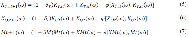
Where;
XT,(ω), XI,it(ω) XMt(ω)=New investments.
δT, δI and δM =Depreciation rates for site-specific tangible and intangible inventories and technology capital, respectively.
φ=Investment adjustment cost control function. In our analysis later, we use the following functional form:

Where;
δ=Depreciation rate of the relevant investment chain.
γY=Trend growth in world output. We then move on to describing the family problem.
Household problem
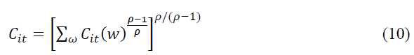
For households in an economic union, i choose the consumption sequence Cit(ω) for all kinds of goods ω, labour supply Li,t, stocks in firms Si,t+1(ω) indexed by ω, bonds Bi,t+1(ω) to solve the following problem:

as
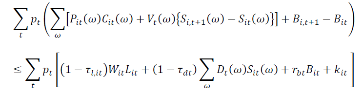
Where
With ρ>0. Here, τIt and τd are the tax rates on employment and profits, τb is the after tax return on international borrowing and lending, Nit is the population in economic union i, and is the externally determined income, which includes both government transfers and net income non-commercial.
“Non-business net income is included so that we can match model calculations with accounts in the data. In our application, we want to distinguish between value added and investment from the commercial and non-trading sectors. We also include non-trading employment as part of total input employment, and this, too, is determined externally. Public consumption is included in Ci.”
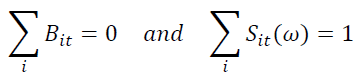
As indicated earlier, the implicit assumption being made is that Ni is the number of production sites and the size of the population. We assume that the productive capacity of an economic union is proportional to the number of the population. Goods purchased from a foreign multinational corporation can either be purchased locally from one of the subsidiaries in i or purchased from the parent company and shipped. By CFit(ω) we denote goods purchased from subsidiaries, where F indicates that they are included in foreign direct investment statistics, and by CFit(ω) we denote goods purchased abroad, where T indicates that they are included in trade statistics. We suppose these goods are not perfect substitutes, but they almost are
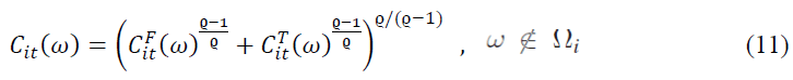
and ϱ ≫ ρ where Ωi states the techniques developed in i. Prices for foreign goods purchased domestically reflect the costs incurred by subsidiaries when operating in i. These costs appear as lower outputs in (3) per unit of compound inputs due to regulatory costs on FDI along the lines of σi<1. Prices for shipped goods include a surcharge given by ζi(ω)Pj(ω), ω ∈ Ωi, if shipped from j to i. Here, we assume that it is not cheaper to ship goods from a subsidiary operating in a third country, (In our quantitative investigation, we treat geographically close countries, such as Canada and the United States, as one region given proximity facilitates intra-firm trade between parents and affiliates).
Market clearing
For each (ω) technique, we require that the following resource constraints remain true:
Where i am home to a multinational company with this technology, i.e., ω ∈ Ωi and j are the economic associations hosting the company's foreign subsidiaries. The market clearing price of the bundle of goods consumed at i, Cit, is determined by
For goods with technology developed abroad, say in union j, the price in i is

Where PFit(ω) is the price of the product in i and PFit(ω) is the price of the product in j plus trade cost, i.e.,
In addition to commodity market clearing, we require asset market clearing, with
For all periods and all companies ω. Finally, we require that labour markets be visible in all economic unions, i.e.,

With total labour supplied by households Lit equal to total labour demanded by firms (ω) and non-business entities Lnb,(ω).
Accounting procedures
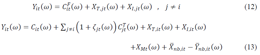
When simulating the model, we compare our theoretical predictions with empirical counterparts in national and international accounts. The most widely used accounting measures are Gross Domestic Product (GDP), Gross National Product (GNP), and the current account components, which are exports, imports, net factor revenues, and net factor payments. In the model, we calculate the nominal GDP as follows:

Where Pnb, is the price index of non-tradable goods, which is subsequently assumed to be an index of prices for the technologies developed in i. Note here that we have subtracted the intangible investments, which are spent by businesses. Although some categories of intangible investments have recently been included in measures of GDP for some countries, most categories are still left out. Given this, we use the old concept of GDP and assume the full cost of intangible investments (we perform a sensitivity analysis to ensure that this assumption does not affect our results).
To calculate the nominal GNP, we need the Net Factor Receipts (NFR) from foreigners and the Net Factor Payments (NFP) for foreigners, which are recorded in the international accounts of i as
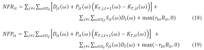
In both expressions, the first amounts are direct investment income from multinational earnings dividends plus retained earnings. The second amounts are portfolio income from household holdings. Finally, the third term is net interest payments, which flow in if positive or out if negative. GNP is the sum of GDP and net factor income (NFR less NFP). In international accounts, the current account is calculated as the sum of net factor income and the trade balance (exports minus imports). The nominal Exports (EX) and Imports (IM) of i are given by
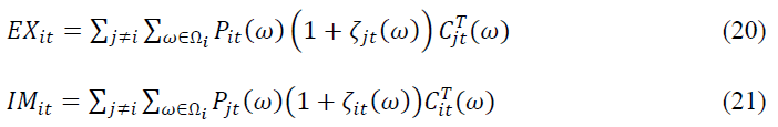
In equilibrium, the net of these values is also equal to GDP minus consumption and tangible investment, which corresponds to the national accounts measure of net exports. Later, we work with real variables. We unpack all nominal variables using the string weighted deflator for one country (which, in our quantitative analysis, is the United States).
Model parameters
In this section, we define model parameters using data from national and international accounts prior to the June 2016 UK referendum. The analysis includes all countries that are major investors in the UK and EU (more specifically, we include the UK and all other EU countries, Norway and Switzerland as a non-EU European region, the United States and Canada as one region, and Japan, Korea and China as one region. All trade flows and foreign direct investment between countries in a region achieved). Parameters are chosen to replicate key statistics, and then the model is used to simulate alternative Brexit scenarios.
Table 1 presents the parameters that are assumed to be identical for all economies. We use co-parameters of family preferences (β, ψ, ρ, ϱ), trend growth in TFP(1+γA)t, trend growth in population (1+γN)t, income shares (Φ, αT, αI), non-business activities (L͞nb, X͞nb/GDP, Y͞nb/GDP), consumption rates (δM, δT, δI), per capita income tax rates on individual (τl, τd), and adjustment costs (φ0, φ1). For all but elasticities ρ and ϱ, we use estimates from the study of McGrattan and Prescott[16], which are reported in Table 1. For substitution criteria governing trade elasticity, we set ρ=10 and ϱ=100. The literature has a wide range of trade elasticity (ρ), from low estimates of 1 to 2 matching quarterly fluctuations in the international business cycle to high estimates of 10 to 15 matching growth after trade liberalization[17,18] for a discussion of a wide range of estimates). Since we are studying Brexit, we used a relatively high estimate, but we later perform sensitivity analysis and repeat our experiments with ρ=5.
| Parameter | Expression | Value |
|---|---|---|
| Preferences Discount factor Leisure weight |
β ψ |
0.981.32 |
| Growth rates (percent) Population Technology |
ϒN ϒA |
1.0 1.2 |
| Income shares (percent) Technology capital Tangible capital Plant-specific intangible capital Labor |
Φ (1-Φ)αT (1-Φ)αI (1-Φ)(1-αT-αI) |
7.0 21.4 6.5 65.1 |
| Non-business sector (percent) Fraction of time at work Investment share Value-added share |
L͞nb X͞nb/GDP Y͞nb/GDP |
6 15 31 |
| Depreciation rates (percent) Technology capital Tangible capital Plant-specific intangible capital |
δM δT δI |
8.0 6.0 0 |
| Tax rates (percent) Labor wedge Dividends |
τl τd |
34 28 |
| Trade elasticities Armington Produced at home versus abroad |
ρ ϱ |
10 100 |
| Adjustment cost parameters Slope Curvature |
φ0 φ1 |
1 2 |
| Note: Parameters are taken from McGrattan and Prescott’s analysis of the US current account, with the exception of trade elasticities and adjustment costs. See the main text for more details. | ||
Table 1. Model parameters common across economies.
And ρ=15. We chose a very high value of ϱ since this is the parameter that governs the substitution between the good sold by the parent company and the good sold by the subsidiary.
Table 2 shows the parameters that differ across economies. The first group shown in panel (a) of Table 2 includes TFP levels, demographics, and corporate profit tax rates. UK GDP and population are normalized to 100, and estimates are set for all other economies relative to that of the UK. The second set of parameters shown in Table 2, panel B, includes all binary openness scores in the pre-Brexit period and is σi0(ω). To keep the analysis traceable and focus on total capital flows, we assume that σi0(ω) is the same for all ω ∈ Ωj, for all i, j with j ≠ i, which means that all MNCs of j face the same constraints on their foreign investment in i (The analysis can be easily expanded if the binary streams are available at a more granular level.) Rows in Table 2, and Panel B represent FDI recipients, and columns represent FDI originators. The third set of parameters that differ for each region shown in Table 2, panel c, are trade costs. Again, rows are recipients and columns are constructors. In the pre-Brexit period, we assume that σi0(ω)=1 and ζi0(ω)=0 for bilateral flows between the UK and the EU, as goods and investments can flow freely within the union.
| United Kingdom | 100 | 100 | 26 | ||
| European Union | 83 | 698 | 23 | ||
| Non-EU Europe | 128 | 20 | 25 | ||
| United States-Canada | 119 | 547 | 34 | ||
| Asia | 40 | 2,418 | 28 | ||
| Panel B. Degrees of openness (σi(ω)) | |||||
| United Kingdom | 1 | 1 | 0.51 | 0.88 | 0.73 |
| European Union | 1 | 1 | 0.90 | 0.87 | 0.72 |
| Non - EU Europe | 0.40 | 0.73 | 1 | 0.64 | 0.57 |
| United States - Canada | 0.77 | 0.84 | 0.81 | 1 | 0.71 |
| Asia | 0.59 | 0.64 | 0.64 | 0.60 | 1 |
| Panel C. Trade costs (ζi(ω)) | |||||
| Technology w from: Shipped to i : | |||||
| United Kingdom | 0 | 0 | 0.00 | 0.14 | 0.02 |
| European Union | 0 | 0 | 0.00 | 0.14 | 0.00 |
| Non-EU Europe | 0.75 | 0.49 | 0 | 0.75 | 0.51 |
| United States-Canada | 0.12 | 0.08 | 0.00 | 0 | 0.00 |
| Asia | 0.53 | 0.42 | 0.12 | 0.52 | 0 |
| Note: The European Union includes all EU countries other than the United Kingdom, non-EU Europe includes Norway and Switzerland, and Asia includes Japan, Korea, and China. All FDI and trade flows between multi-country economies are netted. TFP and population are normalized to 100 for the United Kingdom with other estimates relative to theirs. | |||||
Table 2. Exogenous inputs.
The remaining bilateral openness scores, trade costs, and Trade Direct Transaction (TFP) levels were set to replicate all bilateral FDI flows (relative to GDP), all bilateral trade flows (relative to GDP), and real GDP per capita (Relative to the general (long term growth trend)).
“To define criteria for the degree of openness, we use actual FDI inflows rather than indicators of constraining FDI such as those computed by the organization for economic co-operation and development [19]. The indicators have no theoretical counterpart and cannot accurately measure the overall constraint of a regulatory system. See Appendix to data sources."
After Britain's exit from the European Union (Post-Brixt)
This section uses the parameterized model to analyze several post-Brexit scenarios. In our base scenario, the UK and the EU both raise the costs of foreign investment and trade with each other, effectively dissolving the economic union. To fully understand the forces at play, we begin by analyzing a unilateral move by the United Kingdom to increase costs for foreign investment in the EU, without a change in trade costs. We compare these results to the case of the European union retaliating and imposing the same restrictions on investment in the United Kingdom. We repeat the practice with free movement in foreign direct investment but with higher trade costs, with restrictions imposed first by the United Kingdom and then simultaneously by the European Union. For similar increases in cost, we found welfare losses to be much larger from an increase in FDI costs than from an increase in trade costs because innovation is affected to a greater degree. We then compare the results to the base scenario with costs rising for both FDI and trade, assuming first that the UK acts alone and then assumes that the EU retaliates. In this baseline situation, the well-being of EU citizens is hardly affected if the UK acts alone but suffers significantly if the EU retaliates. The final scenarios consider lower costs of trade and investment in the UK from non-EU countries. In these scenarios, greater openness to outside countries leads to significant welfare gains for the UK.
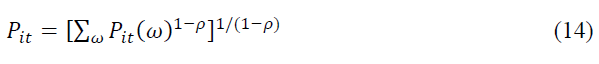
Figure 1 shows the timing of cost changes for the numerical experiments. The actual changes occur two years after the 2016 referendum and are fully phased in by 2022. In the case of higher trade costs, this is the time series of ζi0(ω), with recipient-indexing and ω-source- indexing. For example, if the UK acts alone to restrict trade from EU countries, we feed in the cost increments shown in Figure 1, where the cost starts at 0 (as in item (2, 1) of the matrix in Panel C of Table 2) and eventually rise to 5%. In the case of rising costs on FDI, we use the time series in Figure 1 for 1−σit(ω). For example, when the UK and EU allow mobile investment freely, σit(ω) equals 1. By 2022, the degree of openness for any country that restricts foreign direct investment will be 0.95. In the final section, we alter the timing and magnitude of cost changes and discuss the sensitivity of results to parameter assumptions.

Figure 1. Timing and magnitude of cost increases during transition.
Increasing the costs of foreign direct investment
In Table 3 we analyze one aspect of the post-Brexit transition period: The rising costs of foreign direct investment. For these simulations, the score of the openness parameters in the (2, 1) and then (1, 2) elements of the matrix in Table 2, Panel B, is reduced to 0.95. The first five rows of Table 3, Panels A and B, show the results if the UK tightened restrictions on inward FDI from EU countries and did so unilaterally. The last five rows in both panels show the results if the UK and EU tighten restrictions on each other. The first eleven columns are the percentage changes in current account flows, national account expenditures and labour market variables related to pre-Brexit levels. Two predictions have been reported: The average over the first decade and the change once the economy converges to a new balanced growth path. The latter is shown in parentheses. Welfare, listed in the last column of Panel B, is computed as the consumption equation that should be indifferent between new policies (i.e., higher costs of FDI) and no change. A positive value indicates a gain relative to the pre-Brexit baseline.
First, let's consider the scenario of the UK acting alone to increase costs on incoming FDI from other EU countries. After the announcement, there was a significant drop in FDI inflows into the UK, nearly 43% on average in the first decade. The transition period is about 50 years, and the final decline in FDI inflows into the UK is 16%. During the transition period, trade flows into the UK skyrocketed as companies circumvent increased costs of foreign direct investment. Other effects of cost increases can be better understood if we consider what happens to innovation by multinational companies in the EU and the UK. Higher costs for EU affiliates in the UK affect investment in technology capital as this type of capital can be used non-competitively in multiple locations. If costs are higher on FDI in the EU, then EU companies are at a relative disadvantage in creating new R&D and brands, and so they respond by reducing their investment in XM. If technology capital drops into the UK, British companies respond by increasing their investment in technology capital.
“McGrattan and Prescott[2] work through simple examples to show how country characteristics such as TFP, population, and degree of openness affect predictions about where production occurs and which firms innovate. Because technological capital is non-competitive, there is a magnitude advantage arising from either increased overall productivity to productivity or from more productive locations even if countries are not open to FDI. Countries that are open to FDI can exploit foreign technological capital by allowing direct investment, so the model predicts that those countries that are less Relatively open, are all equal."
In this case, we would expect an average decline in technology capital investment in the EU of 5% relative to pre-Brexit levels during the first decade and 6.4% in the long term. For UK firms, we see the opposite pattern, with an average increase of 2.8% over the first decade and 3.7% over the long term. Although investment in tech capital is higher in the UK, other domestic expenditures are down about 1.6% over the long term, and UK social welfare is less by about 1.9%.
Increased British investment in research and development, brands and other intangible assets is beneficial to the EU as much of this capital can be deployed at no cost in subsidiaries across Europe. Indeed, the trade-off between the higher costs of outward FDI and the higher benefits from British investment is almost formulaic, and EU production and welfare are hardly affected. Basically, the EU reduces investment in technology capital and increases net exports. The EU also benefits from increased investment in other countries' technological capital, which also rises in response to EU divestment. More technology capital means more FDI outward from these countries, especially the United States, Canada and Asia, which benefits all FDI recipients.
| Trade flows | ||||||||
| United Kingdom tightens restrictions on EU FDI unilaterally | ||||||||
| United Kingdom | -42.7 (-16.2) | 1.8 (1.5) | -2.8 (15.5) | 6.2 (32.2) | ||||
| European Union | 1.6 (1.2) | -33.1 (-13.7) | 0.8 (6.6) | 0.4 (5.6) | ||||
| Non-EU Europe | -1.9 (-1.4) | 0.7 (0.4) | 0.6 (-0.6) | -0.4 (-1.4) | ||||
| United States-Canada | -1.3 (-1.1) | 5.1 (2.1) | 0.6 (-1.1) | -1.1 (-1.5) | ||||
| Asia | -1.3 (-0.8) | 3.7 (1.5) | 0.5 (-0.9) | -0.8 (-0.8) | ||||
| United Kingdom and European Union tighten FDI restrictions on each other | ||||||||
| United Kingdom | -37.7 (-11.6) | -80.4 (-34.5) | -0.9 (33.7) | 45.4 (123.3) | ||||
| European Union | -35.4 (-15.3) | -20.7 (-4.6) | 0.8 (34.3) | 2.7 (16.9) | ||||
| Non-EU Europe | -0.5 (0.9) | 22.2 (9.3) | 3.6 (2.0) | -3.6 (-1.2) | ||||
| United States-Canada | -0.1 (-0.1) | 33.9 (13.4) | 4.0 (-4.4) | -6.6 (-5.7) | ||||
| Asia | 2.9 (1.1) | 16.7 (6.2) | 1.3 (1.0) | -2.7 (1.2) | ||||
| Panel B. Expenditures, labor market and welfare | ||||||||
| Labor market | Welfare | |||||||
| United Kingdom tightens restrictions on EU FDI unilaterally | ||||||||
| United Kingdom | -0.2 (-1.6) | -1.7 (-1.7) | -2.0 (-1.6) | -4.7 (-1.6) | 2.8 (3.7) | 1.1 (0.1) | -1.3 (-1.7) | -1.87 |
| European Union | -0.1 (0.0) | 0.1 (0.0) | 0.1 (0.0) | 0.5 (0.0) | -5.0 (-6.4) | -0.1 (0.1) | 0.0 (0.0) | 0.01 |
| Non-EU Europe | 0.0 (0.1) | 0.1 (0.1) | 0.1 (0.1) | 0.5 (0.1) | 0.3 (0.4) | -0.1 (0.0) | 0.1 (0.1) | -0.08 |
| United States-Canada | 0.0 (0.0) | 0.0 (0.0) | 0.1 (0.0) | 0.2 (0.0) | 0.6 (0.8) | 0.0 (0.0) | 0.0 (0.0) | -0.01 |
| Asia | 0.0 (0.0) | 0.1 (0.0) | 0.0 (0.0) | 0.2 (0.0) | 0.1 (0.1) | 0.0 (0.0) | 0.0 (0.0) | 0.00 |
| United Kingdom and European Union tighten FDI restrictions on each other | ||||||||
| United Kingdom | -1.9 (-3.5) | -0.7 (-0.8) | -3.3 (-3.5) | -3.9 (-3.5) | -24.6 (-28.3) | -0.9 (-2.2) | -1.0 (-1.5) | -0.30 |
| European Union | -0.7 (-1.3) | -1.5 (-1.5) | -1.4 (-1.3) | -0.3 (-1.3) | 11.8 (15.9) | 0.6 (0.1) | -1.3 (-1.4) | -2.36 |
| Non-EU Europe | 0.3 (1.1) | 0.4 (0.4) | 0.8 (1.1) | 1.4 (1.1) | 6.0 (6.8) | -0.1 (0.4) | 0.4 (0.6) | 0.30 |
| United States-Canada | -0.1 (0.4) | 0.2 (0.2) | 0.3 (0.4) | 0.9 (0.4) | 3.4 (3.7) | -0.2 (0.1) | 0.1 (0.2) | 0.17 |
| Asia | 0.0 (0.1) | 0.1 (0.1) | 0.2 (0.1) | 0.6 (0.1) | 0.5 (0.5) | -0.1 (-0.1) | 0.1 (0.1) |
0.04 |
| Note: Values reported are percentage changes relative to the pre-Brexit baseline in response to an increase in costs that follows the path shown in Figure 1. Averages over the first decade (years 2016–2025) are displayed first, and changes relative to the eventual balanced growth path are displayed below in parentheses. Changes in output and investments are reported only for businesses. | ||||||||
Table 3. Changes in response to higher FDI costs, relative to pre-Brexit levels.
We find that the quantitative impact of these policy changes critically depends on the relative sizes and TFPs of investing countries and the stock of pre-Brexit FDI.
Next, consider the scenario in which both the UK and the EU raise costs on foreign affiliates with the same size and timing as in the unilateral case. Results are shown in the last five rows of Table 3, Panels A and B. It is not surprising that FDI flows between them fall during the transition period and trade flows increase. UK expenditures of all kinds are falling, with investments in new technology capital falling dramatically. On the new balanced growth trajectory, investment in technology capital, XM, for UK multinationals fell by 28%. In the pre-Brexit period, the model predicts that a significant amount of investment in research and development and other intangible assets is made in the UK because it has a much higher level of TFP than other countries in the union (Table 2, Panel A). Due to the non-competitive nature of technology capital, UK multinationals can use this capital at no cost in many locations within the pre-Brexit union. When production costs rise in the post-Brexit EU, the UK reduces direct investment in other EU locations and instead increases its production funding for non-British multinationals. In fact, foreign investment in the UK is shifting from foreign direct investment to portfolio investment.
With the UK's tech capital declining, the remaining EU countries must raise more of their own, and investment in tech capital is rising by nearly 12% over the first decade, and eventually by 16%. This investment benefits all countries with EU subsidiaries, including the UK. We also see other countries responding with an increase in technology capital investment, which again has a positive impact on all recipients of FDI. As a result, production and FDI outflows are rising in all other regions. On welfare, the UK is worse off at 0.3%, but welfare losses are dampened by increased global innovation. In this case, the EU is in a much worse position, with welfare down 2.4%, due to the loss of capital from the UK.
Increased trade costs
In Table 4 we analyze the second aspect of the post-Brexit transition period the rising costs of trade. To isolate the effect of these costs, we assume no change in FDI costs. As before, we first think of a unilateral move by the UK, and then assume that the EU retaliates. Consider first the results shown in the first five rows of Table 4, panels A and B, for a unilateral policy change. As costs of EU goods shipped to the UK rise, both EU exports and UK imports fall. In the long run, as trade costs rose 5%, EU exports fell 10% and UK imports fell 20%. With cross-commodity substitution, trade flows in other regions increase and foreign direct investment flows increase between the UK and the EU. Because trade costs rise, commodity prices and total expenditures rise, but the quantities consumed and welfare fall. The welfare loss, in this case, is only 0.19%, which is much less than in the case of unilaterally higher FDI costs (Table 3). There is also a modest loss in welfare for the European Union and a modest gain for other regions. If the EU retaliates and raises trade costs on goods shipped from the UK, the results are quantitatively similar to the case with only the UK's policy change. The reason is that in the pre-Brexit period, the UK relied heavily on both EU trade and foreign direct investment, while the EU relied little on UK trade and more on UK foreign direct investment. Thus, lifting barriers against trade from the UK does not change the results much.
| United Kingdom tightens restrictions on EU trade unilaterally | ||||||||
| United Kingdom | 27.5 (9.3) | 1.6 (0.0) | -4.9 (-19.7) | -24.4 (-47.6) | ||||
| European Union | 1.4 (0.2) | 15.1 (5.5) | -7.8 (-14.1) | -3.2 (-9.5) | ||||
| Non-EU Europe | -2.3 (-0.5) | -0.5 (-0.2) | 0.5 (1.6) | 1.8 (3.3) | ||||
| United States-Canada | -1.9 (-0.5) | -0.7 (-0.2) | 2.2 (4.7) | 2.2 (4.8) | ||||
| Asia | 0.5 (0.3) | -1.0 (-0.3) | 0.6 (1.3) | 0.8 (1.3) | ||||
| United Kingdom and European Union tighten trade restrictions on each other | ||||||||
| United Kingdom | 30.2 (10.1) | 3.1 (0.6) | -7.4 (-23.5) | -31.6 (-58.0) | ||||
| European Union | 2.3 (0.5) | 16.2 (5.8) | -9.5 (-16.5) | -4.3 (-11.0) | ||||
| Non-EU Europe | -2.2 (-0.5) | -0.5 (-0.2) | 0.4 (1.5) | (3.1) | ||||
| United States-Canada | -2.1 (-0.6) | -0.9 (-0.3) | 2.7 (5.0) | 2.7 (5.2) | ||||
| Asia | -0.7 (0.0) | -1.2 (-0.4) | 0.8 (1.5) | 1.0 (1.5) | ||||
| Panel B. Expenditures, labor market and welfare | ||||||||
| Labor market | Welfare | |||||||
| United Kingdom tightens restrictions on EU trade unilaterally | ||||||||
| United Kingdom | 1.0 (1.6) | 1.6 (1.6) | 3.2 (1.6) | 7.5 (1.6) | -0.7 (-1.1) | -0.5 (0.0) | 1.5 (1.6) | -0.19 |
| European Union | -0.1 (-0.3) | -0.3 (-0.3) | -0.5 (-0.3) | -1.2 (-0.3) | 0.8 (1.2) | 0.1 (0.0) | -0.2 (-0.3) | -0.04 |
| Non-EU Europe | -0.1 (-0.1) | -0.1 (-0.1) | -0.2 (-0.1) | -0.5 (-0.1 ) | -0.2 (-0.1) | 0.0 (0.0) | -0.1 (-0.1) | 0.07 |
| United States-Canada | 0.0 (0.0) | 0.0 (0.0) | 0.0 (0.0) | -0.1 (0.0) | 0.1 (0.1) | 0.0 (0.0) | 0.0 (0.0) | 0.02 |
| Asia | 0.0 (0.0) | 0.0 (0.0) | 0.0 (0.0) | -0.1 (0.0) | -0.1 (0.0) | 0.0 (0.0) | 0.0 (0.0) | 0.01 |
| United Kingdom and European Union tighten trade restrictions on each other | ||||||||
| United Kingdom | 0.8 (1.5) | 1.5 (1.5) | 2.8 (1.5) | 6.8 (1.5) | -0.3 (-0.8) | -0.5 (0.0) | 1.3 (1.5) | -0.24 |
| European Union | -0.1 (-0.2) | -0.2 (-0.2) | -0.4 (-0.2) | -1.0 (-0.2) | 0.6 (1.0) | 0.1 (0.0) | -0.2 (-0.2) | -0.02 |
| Non-EU Europe | -0.1 (-0.1) | -0.1 (-0.1) | -0.2 (-0.1) | -0.5 (-0.1) | -0.2 (-0.1) | 0.0 (0.0) | -0.1 (-0.1) | 0.07 |
| United States-Canada | 0.0 (0.0) | 0.0 (0.0) | 0.0 (0.0) | -0.1 (0.0) | 0.1 (0.1) | 0.0 (0.0) | 0.0 (0.0) | 0.02 |
| Asia | 0.0 (0.0) | 0.0 (0.0) | 0.0 (0.0) | -0.0 (0.1) | 0.0 (0.0) | 0.0 (0.0) |
0.0 (0.0) |
0.01 |
| Note: Values reported are percentage changes relative to the pre-Brexit baseline in response to an increase in costs that follows the path shown in Figure 1. Averages over the first decade (years 2016–2025) are displayed first, and changes relative to the eventual balanced growth path are displayed below in parentheses. Changes in output and investments are reported only for businesses. | ||||||||
Table 4. Changes in response to higher trade costs, relative to pre-Brexit levels.
Increased costs of foreign direct investment and trade
We now turn to our base scenario with the costs of both foreign direct investment and trade increasing in the post-Brexit era. The results of this case are shown in Table 5, again with the UK unilaterally changing policy and with both the UK and the EU placing restrictions on each other's MNCs. To make the results comparable, we assumed the same timing and magnitude of cost changes as before (Figure 1).
If the UK acts alone, we would expect lower inward FDI and imports due to increased costs, a modest impact on business output, and a 2.4% drop in welfare. Other regions, including the European Union, are responding with adjustments to the current account but do not see a significant welfare impact. As the costs of FDI are higher, the main impact on expenditures is greater investment in technology capital in the UK and to a lesser extent in the EU.
In the base scenario shown in the last five rows of Table 5, panels A and B, with the UK and EU putting up barriers against each other, we expect both to lose out. Welfare in the United Kingdom falls by 1.4%, while in the European union welfare decreases by 2.3%.
“Arkoulakis et al.[11] ran a similar EU exit experiment in a static model without capital normalized for manufacturing data and found real spending losses their measure of change in welfare equal to 1.6% for the UK. In our results, the losses for the remaining EU countries are much smaller. However, since the share of manufacturing value added in GDP is only 9% in the UK, it is not known how large these losses would be if their analysis were extended to all production”.
| Trade flows | ||||||||
| United Kingdom tightens restrictions on EU FDI and trade unilaterally | ||||||||
| United Kingdom | -16.3 (-8.3) | 4.2 (2.2) | -9.2 (-5.7) | -18.2 (-21.3) | ||||
| European Union | 3.4 (1.7) | -20.7 (-10.0) | -6.9 (-8.2) | -3.0 (-4.0) | ||||
| Non-EU Europe | -4.5 (-2.1) | 0.3 (0.3) | 1.2 (0.9) | 1.4 (1.7) | ||||
| United States-Canada | -3.2 (-1.6) | -5.6 (2.4) | 2.8 (2.6) | 0.8 (2.2) | ||||
| Asia | -1.4 (-0.7) | 3.1 (1.3) | 1.1 (0.4) | -0.1 (0.5) | ||||
| United Kingdom and European Union tighten FDI and trade restrictions on each other | ||||||||
| United Kingdom | 7.4 (3.7) | -69.2 (-29.9) | -18.3 (-16.5) | 4.0 (9.1) | ||||
| European Union | -27.3 (-12.0) | -0.6 (1.8) | -10.0 (-1.9) | -5.6 (-5.4) | ||||
| Non-EU Europe | -2.6 (0.2) | 22.2 (9.4) | 4.0 (3.1) | -2.4 (0.8) | ||||
| United States-Canada | -4.8 (-1.6) | 33.4 (13.5) | 7.8 (4.4) | -1.8 (3.1) | ||||
| Asia | -4.9 (-1.5) | 15.4 (5.8) | 2.5 (4.0) | -0.9 (4.3) | ||||
| Panel B. Expenditures, labor market and welfare | ||||||||
| Labor market | Welfare | |||||||
| United Kingdom tightens restrictions on EU trade unilaterally | ||||||||
| United Kingdom | 0.9 (-0.3) | -0.4 (-0.4) | 1.2 (-0.3) | 3.0 (-0.3) | 2.4 (3.2) | 1.0 (0.1) | -0.1 (-0.4) | -2.41 |
| European Union | -0.2 (-0.3) | -0.2 (-0.2) | -0.4 (-0.3) | -0.7 (-0.3) | -4.9 (-6.2) | -0.1 (-0.1) | -0.2 (-0.2) | -0.02 |
| Non-EU Europe | -0.1 (0.0) | 0.0 (0.0) | -0.1 (0.0) | 0.0 (0.0 ) | 0.1 (0.3) | -0.1 (-0.1) | 0.0 (0.0) | -0.03 |
| United States-Canada | 0.0 (0.1) | 0.0 (0.0) | 0.0 (0.1) | 0.1 (0.1) | 0.8 (1.0) | 0.0 (0.0) | 0.0 (0.0) | 0.00 |
| Asia | 0.0 (0.0) | 0.0 (0.0) | 0.0 (0.0) | 0.1 (0.0) | 0.1 (0.0) | 0.0 (0.0) | 0.0 (0.0) | 0.01 |
| United Kingdom and European Union tighten FDI and trade restrictions on each other | ||||||||
| United Kingdom | -1.0 (-3.2) | -0.5 (-0.5) | -2.0 (-3.2) | -2.1 (-3.2) | -23.9 (-26.9) | -0.4 (-2.1) | -0.6 (-1.2) | -1.40 |
| European Union | -0.7 (-1.0) | -1.3 (-1.2) | -1.1 (-1.0) | 0.5 (-1.0) | 10.8 (1.0) | 0.4 (0.1) | -1.1 (-1.2) | -2.32 |
| Non-EU Europe | 0.3 (1.1) | 0.4 (0.4) | 0.6 (1.1) | 0.9 (1.1) | 6.0 (6.9) | -0.1 (0.0) | 0.3 (0.6) | 0.33 |
| United States-Canada | -0.1 (0.4) | 0.2 (0.2) | 0.2 (0.4) | 0.5 (0.4) | 3.7 (4.0) | -0.2 (0.1) | 0.1 (0.3) | 0.19 |
| Asia | 0.0 (0.2) | 0.1 (0.2) | 0.2 (0.2) | 0.5 (0.2) | 0.5 (0.6) | -0.1 (0.0) |
0.1 (0.2) |
0.05 |
| Note: Values reported are percentage changes relative to the pre-Brexit baseline in response to an increase in costs that follows the path shown in Figure 1. Averages over the first decade (years 2016–2025) are displayed first, and changes relative to the eventual balanced growth path are displayed below in parentheses. Changes in output and investments are reported only for businesses. | ||||||||
Table 5. Changes in response to higher FDI and trade costs, relative to Pre-Brexit levels.
As multinational corporations face increased FDI and trade costs, the impact on FDI inflows is not unequivocally negative. Here, it is useful to compare the results of Table 3 with FDI policy changes only and Table 5 with both FDI and trade policy changes. In the latter case, we find an increase in inward FDI of 7.4% in the first decade and 3.7% over the long term, which is in contrast to the predictions of Kierzenkowski et al.,[20]who argue that “lower FDI inflows seem inevitable” if access to the EU single market is restricted. What matters for the outcome is the relative cost of overseas production for shipping abroad. A more predictable outcome, especially when companies invest heavily in technology capital, is lower outward FDI, especially for the UK, which is a smaller country. With their technology capital blocked, UK multinationals innovate less and produce less abroad.
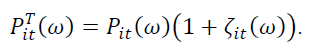
Figure 2 shows the timing of FDI flows between the UK and the EU as a share of the host economy's GNP (As noted earlier, we use the old concept of GNP that excludes intangible investment. If we add all intangible investments, the differences are in the reported proportions less than 0.15% points). Prior to the 2016 referendum, we estimate the ratio of EU investment in the UK to UK GNP at around 1.2%. We estimate the proportion of UK investment in the EU in relation to EU GNP at 1.7%. These pre-Brexit estimates are shown in the figure. After the referendum, we found that UK direct investment in the EU as a share of EU GDP falls to near zero and reaches 1.2% by 2050. Meanwhile, investment in the EU rises before the policy change, and then drops dramatically, before finally bringing investment to near pre-Brexit levels as a share of UK GDP. As trade and investment costs rise in the United Kingdom and the European Union, total business output in these two economies declines. In Figure 2 we show the time series of business output relative to the trends of these economies together with the sum of all others. Thus, before the 2016 referendum, all estimates are zero. Then there is an adjustment period before the costs of FDI and trade actually rise. During that period, business output in the UK and EU rose modestly, because there was significant technical capital still standing. By 2050, UK production is about 3% below trend and EU production is down by about 1%. When aggregated, the business output of businesses outside the UK and abroad is initially below the pre-Brexit level but eventually rises about 0.3% above this level.
Lower costs of foreign direct investment and trade in the UK than outside the EU
Next, we estimate the effect of easing restrictions on foreign direct investment and trade in the UK from other countries, with the same timing as the Brexit timing shown in Figure 1.
We start by assuming that the UK cuts costs only on inflows from the US and Canada and then repeat the exercise for all countries. In both trials, FDI and eventual trade costs were reduced by 5% points compared to the pre-Brexit level.
The results of these experiments are shown in Table 6. The first five rows of panels A and B show the economic impact of lower costs on US and Canadian multinationals exporting to and operating in the UK. These estimates can be directly compared with the baseline scenario shown in the last five rows of Table 5, Panels A and B. It is not surprising that we find greater inflows of foreign direct investment and more imports due to lower costs. Lower FDI costs motivate multinational corporations in the US and Canada to invest more in technology capital and thereby undertake more outward FDI, with an increase of close to 50% above the pre-Brexit level. This increase has a significant impact on welfare in the UK, which is now 0.72% higher. Effectively, the UK is replacing its old partner, which has a relatively low level of TFP, with a new partner which has a higher level of TFP. The change does not affect the EU results much because we assume that they do not open up more to the US or Canada. The last five rows of Table 6, Panels A and B, show the results if costs were reduced for all countries. In this case, another boost to the UK's welfare is now 1.27% higher than the pre-Brexit system. This alternative scenario, which the UK government has discussed as part of its Brexit plan, is clearly better than the base scenario for UK citizens. However, in either case, citizens in the rest of the EU are worse off.

Figure 2. Business outputs of the United Kingdom, European Union, and all other economies.
| United Kingdom lowers restrictions on United States | ||||||||
| United Kingdom | 26.3 (13.8) | -71.1 (-30.9) | -11.3 (-18.2) | 10.9 (-7.1) | ||||
| European Union | -26.7 (-11.7) | -10.1 (-2.3) | -12.2 (-3.6) | -5.5 (-6.3) | ||||
| Non-EU Europe | -2.3 (0.3) | 22.1 (9.5) | 3.6 (2.8) | -2.8 (0.0) | ||||
| United States-Canada | -8.9 (-3.4) | -49.2 (21.3) | 12.2 (7.3) | 2.1 (4.2) | ||||
| Asia | -5.1 (-1.6) | 12.1 (4.5) | 1.8 (3.8) | -0.7 (3.9) | ||||
| United Kingdom lowers restrictions on all but European Union | ||||||||
| United Kingdom | 32.9 (17.1) | -71.3 (-31.0) | -9.5 (-20.1) | 11.1 (-10.2) | ||||
| European Union | -26.7 (-11.8) | -12.3 (-3.2) | -12.4 (-3.6) | -5.4 (-6.3) | ||||
| Non-EU Europe | -2.3 (0.3) | 22.6 (9.8) | 3.6 (2.4) | -2.7 (-1.0) | ||||
| United States-Canada | -9.0 (-3.5) | 47.8 (20.7) | 12.1 (7.5) | 2.1 (4.4) | ||||
| Asia | -5.5 (-1.7) | 30.2 (12.8) | 2.0 (3.2) | 0.1 (2.7) | ||||
| Panel B. Expenditures, labor market and welfare | ||||||||
| United Kingdom lowers restrictions on United States | ||||||||
| United Kingdom | -1.9 (-2.3) | 0.3 (0.5) | -2.8 (-2.2) | -4.3 (-2.2) | -25.9 (-29.3) | -1.6 (-2.1) | -0.3 (-0.2) | 0.72 |
| European Union | -0.8 (-1.2) | -1.5 (-1.3) | -1.3 (-1.2) | 0.2 (-1.2) | 9.0 (12.3) | 0.5 (0.0) | -1.3 (-1.3) | -2.39 |
| Non-EU Europe | 0.1 (1.0) | 0.2 (0.4) | 0.4 (1.0) | 0.7 (1.0 ) | 5.9 (7.0) | 0.0 (0.4) | 0.2 (0.5) | 0.33 |
| United States-Canada | 0.0 (0.6) | 0.1 (0.3) | 0.3 (0.6) | 0.6 (0.6) | 5.6 (6.5) | -0.1 (0.1) | 0.1 (0.4) | 0.25 |
| Asia | -0.1 (0.1) | -0.1 (0.1) | 0.0 (0.1) | 0.3 (0.1) | 0.3 (0.4) | -0.1 (-0.1) | -0.1 (0.1) | 0.04 |
| United Kingdom lowers restrictions on all but European Union | ||||||||
| United Kingdom | -2.1 (-1.8) | 0.7 (0.8) | -2.8 (-1.8) | -4.1 (-1.8) | -26.4 (-29.9) | -2.0 (-2.1) | -0.1 (0.1) | 1.27 |
| European Union | -0.8 (-1.2) | -1.5 (-1.3) | -1.3 (-1.2) | 0.2 (-1.2) | 8.6 (12.0) | 0.5 (0.0) | -1.3 (-1.3) | -2.41 |
| Non-EU Europe | 0.2 (1.0) | 0.2 (0.4) | 0.4 (1.0) | 0.6 (1.0) | 6.0 (7.2) | 0.0 (0.4) | 0.2 (0.5) | 0.32 |
| United States-Canada | 0.0 (0.6) | 0.1 (0.3) | 0.3 (0.6) | 0.6 (0.6) | 5.5 (6.3) | -0.1 (0.1) | 0.1 (0.4) | 0.24 |
| Asia | -0.1 (0.1) | -0.1 (0.1) | 0.0 (0.1) | 0.2 (0.1) | 0.7 (0.9) | 0.0 (-0.1) | -0.1 (0.1) | 0.07 |
| Note: Values reported are percentage changes relative to the pre-Brexit baseline in response to an increase in costs that follows the path shown in Figure 1. Averages over the first decade (years 2016–2025) are displayed first, and changes relative to the eventual balanced growth path are displayed below in parentheses. Changes in output and investments are reported only for businesses. | ||||||||
Table 6. Changes in response to lower FDI and trade costs into the United Kingdom from other nations in the baseline scenario, relative to pre-Brexit levels.
Sensitivity
To assess the significance of policy and parameter experiments, we re-ran the basic numerical experiment described in the last five rows of Table 5, Panels A and B, reporting the main statistics for the UK in Table 7, and we also ran experiments in the more general model of Holmes, McGrattan, and Prescott[16]. In the first three alternatives, we vary the timing and magnitude of the policy changes shown in Figure 1. In the first case, the initiation of cost increases is delayed by two years relative to the base case. In the second, we assume that restrictions tightened at a slower pace, with costs falling taking about two more years. In the third case, we assume that the final costs differ by 10%, which is a multiple of the base case. Delays and slow additions affect averages over the first decade, but not much. The doubling of costs has a near-multiple effect on investment in technology capital and welfare, but less so on current account and production.
In the remaining alternatives listed in rows 5 to 10 of Table 7, we change the parameters of the model. First, we broaden the concept of a trade by including both trade in goods and services when calibrating trade costs. Since the services trade is still relatively small, this doesn't change our results much. Second, we change the Armington elasticity ρ, first decreasing it to ρ=5 (row 6) and then increasing it to ρ=15 (row 7), to cover the wide range of estimates in the literature. Changes in this variable affect imports and inward FDI in predictable ways: when elasticity is high, inflows are more sensitive to changes in policy as consumers are more likely to respond to higher priced foreign goods by substituting for domestically produced goods. Similarly, increased sensitivity to trade costs means that multinational companies are more likely to produce their commodity in a foreign country than to ship it. Therefore, in the case of higher elasticity, we see that inward FDI increases even more than in the base case. If we reduce the substitution elasticity between foreign goods produced by the subsidiaries and those produced by the parents to ϱ=10, we find a much larger welfare loss for the UK when the costs of foreign goods, whether produced in the UK or abroad, go up. In this case, summarized in row 8, pre-Brexit UK consumption has a much smaller domestic share, and thus the negative impact of higher costs on foreign goods during the post-Brexit period is greater.
| Inward FDI | Imports | Business output | Technology investment | Welfare | |
|---|---|---|---|---|---|
| Baseline | 7.4 (3.7) | -18.3 (-16.5) | -1.0 (-3.2) | -23.9 (-26.9) | -1.40 |
| Delay Brexit | 13.4 (3.7) | -13.5 (-16.3) | -0.7 (-3.2) | -21.4 (-26.9) | -1.33 |
| Slower phase-in | 10.5 (3.7) | -16.2 (-16.4) | -0.9 (-3.2) | -22.6 (-26.9) | -1.37 |
| Double costs | 7.5 (5.8) | -31.7 (-26.4) | -1.6 (-6.2) | -44.8 (-48.0) | -2.94 |
| Broaden scope | 6.8 (3.6) | -16.4 (-14.7) | -0.9 (-3.2) | -24.0 (-26.9) | -1.38 |
| Decrease elasticity | -2.1 (-2.5) | -10.3 (-2.8) | -0.6 (-1.7) | -13.6 (-13.1) | -1.69 |
| Increase elasticity | 14.7 (9.6) | -24.1 (-27.2) | -1.2 (-4.6) | -31.6 (-38.8) | -1.14 |
| Set elasticities equal | 24.3 (8.6) | -11.1 (-15.5) | -2.4 (-5.0) | -24.6 (-26.9) | -3.04 |
| Lower capital share | -10.4 (-17.9) | -14.2 (7.1) | -1.5 (0.2) | -25.0 (-28.5) | -1.58 |
| No adjustment costs | 12.9 (3.6) | -23.3 -16.0) | -1.3 (-3.4) | -33.1 (-27.0) | -1.23 |
| Note: Values reported are percentage changes relative to the pre-Brexit baseline in response to an increase in costs that follows the path shown in Figure 1. Averages over the first decade (years 2016–2025) are displayed first, and changes relative to the eventual balanced growth path are displayed below in parentheses. Changes in output and investments are reported only for businesses. The baseline implementation corresponds to the last five rows of Table 5, Panels A and B. The “delay Brexit” assumes a two-year delay in implementation. The “slow phase-in” assumes that Brexit occurs at the same time as the baseline but takes two years longer to be phased in. The “double costs” assumes that long- run costs rise to 10 percentage points. The “broaden scope” uses trade data on services as well as goods to parameterize the model. The “decrease elasticity” uses an Armington elasticity of ρ=5. The “increase elasticity” uses an Armington elasticity of ρ=15. The “set elasticities equal” uses ϱ=ρ=10. The “lower capital share” uses φ=0.01. The “no adjustment costs” turn off all costs of adjusting capital. | |||||
Table 7. Changes in UK aggregates relative to pre-Brexit levels (alternative policies and parameters).
We're also rerunning numerical experiments with lower shares of technology capital. The case with φ=0.01 is reported in row 9 of Table 7. If we compare these results with the base case in row 1, we see that changes in projected FDI inflows have opposite signs. This is to be expected as φ approaches zero because firms invest less in R&D and other intangible assets and thus have less incentive to engage in FDI than in the base case, especially with higher regulatory costs. On the new balanced growth path, we find smaller changes in UK production and little reallocation of global production, since investment of technology capital, is a critical factor in who produces and where. Finally, although not shown in the table, we found that greater openness to non-EU countries (as in the trials shown in Table 6) does not lead to positive welfare gains for the UK, as we found at baseline. The positive gains in the case of φ=0.07 derive from large increases in intangible investment and increased outward FDI by non-EU countries in the post-Brexit period.
In the last row of Table 7, we re-run the numerical experiment with no modification costs. As expected, there are larger initial responses because the investment is adjusted immediately after the policy is announced. In fact, some balance investments fall below negative, which is why they are included in the baseline criteria. However, the results are not significantly different from the baseline.
Data supplement
In this appendix, we report our data sources. All data and computer codes can be found at www.econ.umn.edu/∼erm.
The main series used in our analysis are population, GDP, foreign direct investment flows, trade flows, and average corporate tax rates. The source of population and GDP is the World Bank's World Development Indicators (WDI) database[21]. The specific series we use is total population (SP.POP.TOTL), GDP in current US dollars (NY.GDP.MKTP.CD), and GDP at purchasing power parity in constant 2011 international dollars (NY.GDP.MKTP). PP.KD). For each of these variables, when constructing composite countries, such as the European Union or the United States plus Canada, we simply add the population and GDP across the countries to arrive at the total for the composite country.
The main source of bilateral FDI inflows is FDI statistics from the Organization for Economic Co-operation and Development (OECD). These flows are reported to the OECD by the member states of each of its partner countries. The data on FDI inflows into China from its partners comes from the China Statistics Yearbook[22]. These data are available from 1990 to 2013. Data for outbound FDI by host country are available from the China trade yearbook[23] for the years 2003-2013. When constructing total FDI statistics for composite country groups, we subtract any cross flows of FDI between countries that are members of these groups.
We use two sources of bilateral trade flows: The UN Comtrade database and the global input-output database[24]. In the main calibration, we use Comtrade data, which includes merchandise trade only. We collect data on total imports (flow=6) and total exports (flow=5) between countries, where trade is reported using ISIC 3 review nomenclature. In our sensitivity analysis, we use data from the global input-output database, which is available from from 1995 to 2012, it includes trade in goods and services. Annual tables provided by the global input-output database show how much of a good country A produces in a given industry and country B uses, by category or end-use industry. In order to establish total bilateral flows of exports from country A to country B, we aggregate data across all production industries by country A and all usage categories by country B. In both cases, we group the data into the five composite country groups. Similar to our construction of bilateral FDI flows, we construct all flows of a composite country group by adding up all imports (exports) to (outside) countries within the composite country and subtracting any flows within a group of countries from the total. In addition, we use bilateral trade data to generate total imports (exports) from the other countries in the model.
Data on corporate tax rates are from estimates from the accounting firm KPMG International[25-35]. In order to establish tax rates for our composite countries, a simple average is taken across the tax rates prevailing in the countries being aggregated. To calculate the initial steady state, each data series was averaged over three years: 2010 through 2012. We chose a start date of 2010 to avoid the Great Recession drop and an end of 2012 because that was the last year for which all data series were available.
In this paper, we estimate the impact of tightening regulations on trade and foreign direct investment of foreign multinational firms after the UK referendum to leave the European union. We show that the impact on investment, production and welfare depends significantly on whether the UK acts unilaterally to block EU inflows or jointly with EU countries to erect cross border barriers on each other. Economies that remain open enjoy the benefit of new ideas and knowledge of others without making costly investments themselves. If the UK unilaterally tightens regulations, British companies have to invest on their own, and UK citizens will be much worse. Although it's exports and foreign direct investment face higher costs, the EU benefits from increased investment by British companies in research and development and other intangible capital.
If the EU also tightens regulations on trade and foreign direct investment from the UK, the relative sizes and TFP of the two economies, along with those of other investing nations, will determine global investment and production patterns in the post-Brexit period. Given that the UK is relatively small if UK and EU companies face the same stricter regulations, we expect that the optimal response for UK companies is to reduce investment in research and development and other intangible assets and to divest in their EU subsidiaries. We expect that the optimal response for UK citizens will be to increase international lending by financing the production of multinational companies from outside the UK, both domestically and abroad. In this scenario, we estimate large welfare losses for both the UK and other EU countries. However, we would appreciate a significant welfare gain for UK citizens if their government were to simultaneously reduce existing restrictions on large investors outside the EU.