Lakshmi Kameswari Gangaraju1*, Srinivas Sharma Gangaraju2
1 Department of Mathematics, Applied Sciences & Humanities, Maturi Venkata Subba Rao Engineering College, Nadergul, Telangana, India
2 Department of Automobile Engineering, Maturi Venkata Subba Rao Engineering College, Nadergul, Telangana, India
Received: 04-May-2022, Manuscript No. JSMS-22-66442; Editor assigned: 06-May-2022, Pre QC No. JSMS-22-66442 (PQ); Reviewed: 20-May-2022, QC No. JSMS-22-66442; Revised: 27-May-2022, Manuscript No.JSMS-22-66442 (A); Published: 03-Jun-2022, DOI: 10.4172/J Stats Math Sci.8.5.005.
Visit for more related articles at Research & Reviews: Journal of Statistics and Mathematical Sciences
Estimation of productivity is the measure of performance of plant which is invariably affected by labour, capital and other dependent resources (mostly psychological, social, economic, regional and environmental aspects). In India, the major electricity production is by coal and as per recent statistics report of Govt.of.India; the coal production has drastically increased due to high demand. Regression method is adopted to estimate the production function of coal mines and isoquant, isocost curves are drawn to understand the capital and cost involved in the production of coal. Total factor productivity is estimated using the CD production function approach.
Total productivity model; Partial productivity; Machine productivity; Isoquant; Parameters
Coal is a major source of energy generation in India, where about 60% of total electricity is generated using coal. The coal is mined from the open cast and under mines. The coal available in India is mostly lignite and various companies under ministry of coal, GOI, mine the coal. Though major industrial equipment is used for production of coal, labour play a major role in coal mining. Sumanth developed a productivity measurement model that considers the impact of all input factors on the output in a tangible sense [1]. The model is applicable not only as an aggregate tool at the firm level, but it can also be used at an operational unit level. Total Productivity Model (TPM) is a basic model from which several versions are derived. It is based on total productivity measure and a set of five partial productivity measures. The model can be applied in any manufacturing company or any service organization. One of the approaches used by Total Productivity model is production functions approach.
“Productivity needs to be viewed as one of a group of performance criteria against which managers can assess, evaluate and base decisions regarding the organizational systems they are managing”. Productivity is defined as the ratio of output to input of the production system. Based on the type of input used, the productivity can be classified as Total productivity, machine productivity and partial productivity. Total productivity is defined as the ratio of output to total inputs. It is expressed as:
Total Productivity=Output/Input
Measuring productivity is difficult because the inputs such as materials, machines and energy have different values and different physical units. Due to different units of input it is difficult to interpret the effect of each input on the productivity. This is overcome by partial productivity. Partial productivity is defined as the ratio of output to individual input. It is expressed as:
Partial Productivity=Output/Individual Input
Machine Productivity=Output Production Quantity/Machine Input
There are many criteria to measure the machine productivity based on the type of machine input such as number of machines or total processing time. For measuring productivity at company level, there are different approaches taken by economists, engineers, managers, and accountants. Some of them are index approach, production function approach, input-output approach, utility approach, servo-system approach, array approach, financial ratios approach, capital budgeting approach and unit cost approach.
As per pure theory of production functions, Cobb-Douglas function and Constant elasticity of substitution are two important functions in estimation of productivity. The Cobb-Douglas production function can be expressed as:
Y=A * La * K (1-a)
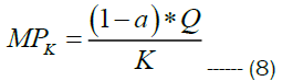
Where: Y is real output (Quantity of goods produced ), A is a scalar known as Total Factor Productivity, L is a measure of labour input, K is a measure of capital input, “a” is a fractional exponent, 0<a<1, representing labour's share of output. For constant scale of returns a+b=1; Hence b=1-a. Total factor productivity is rewritten as A=Y/(La * K (1-a)) from Cobb Douglas production function. Hence Total Factor productivity maximizes the quantity of products produced for same value of capital and labor. The Cobb-Douglas production function has the property of constant returns to scale, which indicates that any proportional increase in both inputs results in an equal proportional increase in output. The Constant Returns to Scale property occurs because the sum of the exponents on the L and K input variables sum to one.
Re-writing the production function, one obtains
A=Y/La * K (1-a)
This expression is referred to as a measure of total factor productivity; that is, the scalar A has an economic meaning. The denominator is a geometric-weighted average of the inputs used to produce real output. Thus, A can be interpreted as real output per unit of input. This is a better measure of productivity when compared to Y/L, Y/K, or Y/l and which are measures of partial productivity. Partial productivity measures do not take into account the possibility of differing amounts of other inputs used in production which might account for the greater or lesser productivity of a single input.
Marginal product of labour and capital
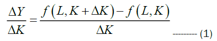
For a given amount of labor and capital, the ratio  is the average amount of production for one unit of capital. On the other hand the change in the production when the labor is fixed and the capital is changed from K to K + ΔK is ΔY=f(L, K + ΔK) − f(L, K).
Dividing this quantity by ΔK gives the change in the production per unit change in capital, given by
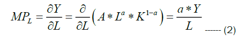
This is written as  and denoted by MPL. For Cobb Douglas production function, the MPL is given by
Isoquant of production function
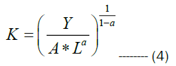
The production function Y=f(L,K) describes a set of inputs in terms of labour and capital. An Isoquant represents the relation between labour and capital input for a certain level of quantity. It is a line having downward slope indicating the relation between labour and capital for constant quantity output. For a given value of output Y, the value of capital K for different values of Labour is arrived using the relation
The slope of an isoquant is referred to by some economists as the Marginal Rate of Substitution (MRS). Other authors in the area of econometrics refer to it as the rate of technical substitution (RTS) or the Marginal Rate of Technical Substitution (MRTS). Suppose the production function is a Y=f(x1, x2), where x1 and x2 are inputs then isoquant represents as shown in Figure 1.

Figure 1: Preferred choice of higher learning institution.
Profit maximization by Cobb Douglas production function
A production function is a heuristic that specifies how much quantity (preferably maximum output) that can be
produced from various combinations of inputs. In general a production function is mathematically written as  Such that Y=f(X), where X is a vector of factor inputs (X1, X2, X3… Xn)1 and f(X) is the maximum
output that can be obtained from the given set of inputs Xi∈R+.This is applicable for estimating production
econometrics at individual level and at total level. One of the methods involved is Elasticity of substitution. Elasticity
of substitution in production is a measure of how easy it is to shift between factor inputs, typically labor and capital.
This measure is defined as the percentage change in factor proportions resulting from a one-unit change in the
Marginal Rate of Technical Substitution (MRTS).
Such that Y=f(X), where X is a vector of factor inputs (X1, X2, X3… Xn)1 and f(X) is the maximum
output that can be obtained from the given set of inputs Xi∈R+.This is applicable for estimating production
econometrics at individual level and at total level. One of the methods involved is Elasticity of substitution. Elasticity
of substitution in production is a measure of how easy it is to shift between factor inputs, typically labor and capital.
This measure is defined as the percentage change in factor proportions resulting from a one-unit change in the
Marginal Rate of Technical Substitution (MRTS).
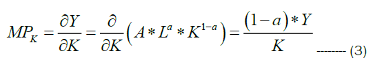
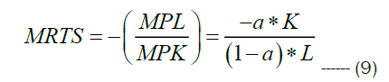
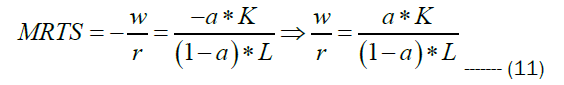
MRTS is the rate at which labor can be substituted for capital while holding output constant along an isoquant; that is, it is the slope of the isoquant at a given point. Thus, for a two-input production function, Y=f (K, L), the elasticity of substitution between capital and labor is given by MRTS=-(MPL/MPk); where MPL and MPK are marginal productivity of labour and capital. Hence for Cobb Douglas production function MPL and MPK are given by the following relations
This implies that
Hence Marginal rate of technical substitution is given by
If the cost function 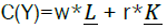 then MRTS as per fundamental definition is also looked as
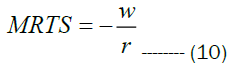
Where w indicates the wages of labour and r is the capital while holding constant quantity (or output).
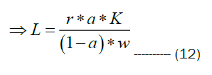
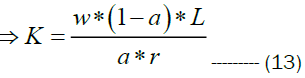
Substituting the optimality condition capital from equations 14 in equation 15 we have
Similarly substituting the optimality condition of labour from equation 12, we have
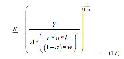
Hence the cost function is written as
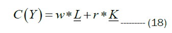
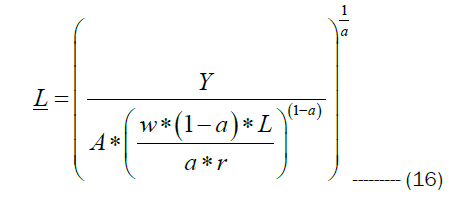
Substituting the conditional demands of labour and capital in the cost function given by the expression 18, we have
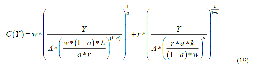
If P(Y) is the price of output, then the profit function is given by the relation
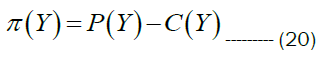
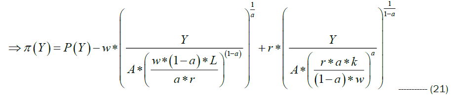
Hence  is dependent on index of Labour, Total factor productivity A and price of output.
Productions functions are first introduced by Cobb-Douglas in their working paper of American economic association suggested that there is a need for measuring the volume of physical production by considering two factors [2]. First to measure the changes in amount of labour and capital to produce the volume of physical production and secondly the relationship between capital, Labour and volume of physical production (Quantity of goods). In the last 30 years several economists have developed various mathematical/stochastic procedures for improving productivity by production functions approach. James Levinsohn, in his working paper introduced a new method for conditioning out serially correlated unobserved shocks to the production technology by building ideas first developed in Olley and Pakes [3,4]. Olley and Pakes showed how to use investment to control for correlation between input levels and the unobserved firm specific productivity process. They have proved that investment; intermediate inputs (those inputs which are typically subtracted out in a value-added production function) solve the duality of problem and highlighted three potential advantages to using an intermediate inputs approach relative to investment. Zellener have presented two alternative specifications of the Cobb-Douglas production function model [5]. The first was referred to as the "traditional model," which assumes that firms operate on a non-stochastic production function and maximize profits. The model is then made stochastic by introduction of random disturbance terms by the econometrician, which yields the traditional or Marschak-Andrews' model. The second model involves assuming that the production functions of firms are identical in form and parameters are concerned and, in addition, are stochastic. In this model, the profit function is random, and they have assumed that firms maximize the mathematical expectation of profits, an assumption that leads to a new model for which estimating techniques have been presented. Kyoo il Kim has revisited the production function estimators of Olley and Pakes and Levinsohn and concluded that they have used control functions to address the simultaneous determination of inputs and productivity, by assuming input demand is a monotonic function of productivity holding capital constant [6]. If the observed capital variable is measured with error, input demand will not generally be monotonic in the productivity shock holding observed capital constant. Kyoo il Kim has developed consistent estimators of production function parameters in the face of this measurement error [7].
The coal mining data is collected from the web, as the wages payment and labour involved are strictly confidential [8]. As per the existing labour laws, the minimum wage payment is assumed and appropriately data is selectively segregated for analysis. The various coal mining companies’ yearly production data is collected and re-estimated on monthly basis. In India, as per ministry of coal, there are more than 75 coal mining companies and 35 top coal companies, which mine the coal in open cast and under earth deep excavation . The plant ID, Quantity produced in Tonnes per month, labour in hours and capital in Lakhs of INR is presented below (Tables 1-5) (Figures 2 and 3).
| Plant | Coal Production ( In thousand tons) | Labour ( In hours) | Capital ( In Lakhs) |
|---|---|---|---|
| 1 | 61.07 | 500 | 100 |
| 2 | 48.9 | 669 | 125 |
| 3 | 126.38 | 789 | 124 |
| 4 | 144.08 | 1236 | 178 |
| 5 | 121.17 | 2344 | 150 |
| 6 | 151.22 | 1590 | 190 |
| 7 | 198.19 | 2895 | 256 |
| 8 | 142.92 | 3546 | 198 |
| 9 | 92.08 | 1233 | 134 |
| 10 | 103.28 | 1459 | 165 |
Table 1. Coal production and its data.
| Plant | Coal Production (In thousand tons) | Labour (In hours) | Capital (In Lakhs) | Ln (Q) | Ln (L) | Ln (K) |
|---|---|---|---|---|---|---|
| 1 | 61.07 | 500 | 100 | 4.11195 | 6.2146 | 4.60517 |
| 2 | 48.9 | 669 | 125 | 3.88978 | 6.5058 | 4.82831 |
| 3 | 126.38 | 789 | 124 | 4.8393 | 6.6708 | 4.82028 |
| 4 | 144.08 | 1236 | 178 | 4.97034 | 7.1196 | 5.18178 |
| 5 | 121.17 | 2344 | 150 | 4.79722 | 7.7596 | 5.01064 |
| 6 | 151.22 | 1590 | 190 | 5.01877 | 7.3715 | 5.24702 |
| 7 | 198.19 | 2895 | 256 | 5.28922 | 7.9707 | 5.54518 |
| 8 | 142.92 | 3546 | 198 | 4.96228 | 8.1736 | 5.28827 |
| 9 | 92.08 | 1233 | 134 | 4.5227 | 7.1172 | 4.89784 |
| 10 | 103.28 | 1459 | 165 | 4.6374 | 7.2855 | 5.10595 |
Table 2. Regression Analysis for estimation of total factor productivity.
| Regression Statistics | |
|---|---|
| Multiple R | 0.834506 |
| R Square | 0.696401 |
| Adjusted R Square | 0.609658 |
| Standard Error | 0.268078 |
| Observations | 10 |
Table 3. Various form of Regression statistics.
| ANOVA | df | SS | MS | F | Significance F |
|---|---|---|---|---|---|
| Regression | 2 | 1.153926 | 0.576963 | 8.028351 | 0.015419 |
| Residual | 7 | 0.50306 | 0.071866 | ||
| Total | 9 | 1.656987 |
Table 4. Significance of ANOVA.
| Coefficient | Standard Error | t Stat | P-value | Lower 95% | Upper 95% | Lower 95.0% | Upper 95.0% | |
|---|---|---|---|---|---|---|---|---|
| Intercept | -1.40085 | 1.79119 | -0.78208 | 0.459801 | -5.63634 | 2.83464 | -5.63634 | 2.83464 |
| Ln(L) | 0.144941 | 0.268792 | 0.539229 | 0.606446 | -0.49065 | 0.780534 | -0.49065 | 0.780534 |
| Ln(K) | 1.001067 | 0.618841 | 1.617646 | 0.149772 | -0.46226 | 2.464394 | -0.46226 | 2.464394 |
Table 5. Production function data

Figure 2: Isoquant curves representing labour and capital. Note:

Figure 3: Isoquant with Isocost. Note:
Linear regression method is used with estimate the total factor productivity, using the logarithmic function for the data shown in Table 1.
The Production function for the above data is obtained as Q=0.246*(L)0.6 *(k)0.4
The dotted line indicated above in the Figure 2 is isocost drawn to 250,000 tonnes of coal production which indicates that 350 hours of labour with 30000 lakhs of capital produce the required quantity of coal which is more capital intensive. The isocost line is again drawn for the ciurve producing 250,000 tonnes of coal, with 10000 lakhs of capital and 600 hours of labour, which is labour intensive (Figure 4) (Table 6).
| Plant | Coal Production ( In thousand tons) | Labour (In hours) | Capital (In Lakhs) | Ln (Q) | Ln (L) | Ln (K) | TFP | MPL | MPK | MRTS |
|---|---|---|---|---|---|---|---|---|---|---|
| 1 | 61.07 | 500 | 100 | 4.11 | 6.21 | 4.61 | 0.25 | 0.07 | 0.24 | 0.3 |
| 2 | 48.9 | 669 | 125 | 3.89 | 6.51 | 4.83 | 0.25 | 0.04 | 0.16 | 0.28 |
| 3 | 126.38 | 789 | 124 | 4.84 | 6.67 | 4.82 | 0.25 | 0.1 | 0.41 | 0.24 |
| 4 | 144.08 | 1236 | 178 | 4.97 | 7.12 | 5.18 | 0.25 | 0.07 | 0.32 | 0.22 |
| 5 | 121.17 | 2344 | 150 | 4.8 | 7.76 | 5.01 | 0.25 | 0.03 | 0.32 | 0.1 |
| 6 | 151.22 | 1590 | 190 | 5.02 | 7.37 | 5.25 | 0.25 | 0.06 | 0.32 | 0.18 |
| 7 | 198.19 | 2895 | 256 | 5.29 | 7.97 | 5.55 | 0.25 | 0.04 | 0.31 | 0.13 |
| 8 | 142.92 | 3546 | 198 | 4.96 | 8.17 | 5.29 | 0.25 | 0.02 | 0.29 | 0.08 |
| 9 | 92.08 | 1233 | 134 | 4.52 | 7.12 | 4.9 | 0.25 | 0.04 | 0.27 | 0.16 |
| 10 | 103.28 | 1459 | 165 | 4.64 | 7.29 | 5.11 | 0.25 | 0.04 | 0.25 | 0.17 |
Table 6. Estimation of Marginal return of technical substitution.

Figure 4: Isoquant with changed slope of isocost line. Note:
The marginal productivity of Labour and capital with marginal return of technical substitution are estimated and presented.
Students were found to be more motivated to learn probability and statistics with the use of school gardens. Similarly, they pointed out that they could see the relevance and use that they could give to statistics and probability by applying them to the process and work with school gardens. In the present work Isoquants and Isocost lines with production function are estimated for coal mining industry. The decisive parameters for arriving at labour intensive and capital intensive charts are performed. Regression analysis with 95% of confidence level is performed and total factor productivity is estimated.
[Crossref]