Research & Reviews: Journal of Material Sciences
ISSN:2321-6212
ISSN:2321-6212
Duan QQ1,2, Pang JC1*, Zhang P1, Li SX1 and Zhang ZF1*
1Shenyang National Laboratory for Materials Science, Institute of Metal Research, Chinese Academy of Sciences, Shenyang 110016, P. R. China
2University of Chinese Academy of Sciences, 19 Yuquan Road, Beijing 100049, China
Received Date: Dec 08, 2017; Accepted Date: Dec 27, 2017; Published Date: Jan 9, 2018
Copyright: © 2018 Duan QQ, et al. This is an open-access article distributed under the terms of the Creative Commons Attribution License, which permits unrestricted use, distribution, and reproduction in any medium, provided the original author and source are credited.
DOI: 10.4172/2321-6212.1000207
Visit for more related articles at Research & Reviews: Journal of Material Sciences
S-N curves of AISI 4340 and SCM 435 steels were determined according to the qualifications and systematically investigated by Basquin relation. The change of parameters (fatigue strength coefficients and exponents) of these S-N curves with increasing tensile strength was analyzed and summarized. For the steels with the same type of S-N curves, as tensile strength increases, their fatigue strength coefficients linearly increase and fatigue strength exponents almost keep unchanging at first and then decrease linearly. In addition, the fatigue mechanisms controlling the parameters of SN curves with tensile strength increasing were discussed. It is briefly explained that the fatigue strength coefficient can be improved by strengthening mechanisms, and the change of fatigue strength exponent with tensile strength may be influenced by the change of fatigue crack initiation sites, the microstructures and fatigue fractographies of steels treated by different heat treatments. Through properly adjusting fatigue strength coefficients and fatigue strength exponents the fatigue strength can be improved in the course of the selection and preparation of steels.
Steels, Parameters of S-N curve, Tensile strength, Fatigue mechanism
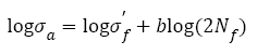
Fatigue curve, named S-N curve, is defined as the regression of stress range with increasing fatigue lifetime. For high/ very high cycle fatigue, S-N curve is a principal reference to determine fatigue strength and design criterion. In the middle 1800s, fatigue failures obviously increased because of the industrial revolution, S-N curve was initially developed by W hler, therefore, in honor of him, S-N curve was also called W hler curve since 1936 [1,2]. Incidentally, his experimental results were expressed in the form of tables at that time, only his successor Spangenberg plotted them as curves in the unusual form of linear abscissa and ordinate [2]. Not until 1910 did Basquin represented them in the form of logarithm ordinate and abscissa and found the simply linear formula such that
 (1)
(1)
Where, σa is stress amplitude,  is the fatigue strength coefficient, Nf is the number of cycles to failure, 2Nf is the number of reservals to failure and b is the fatigue strength exponent on a log-log plot and also named as Basquin exponent. Eqn. (1) can be written as an exponential format:
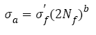 (2)
(2)
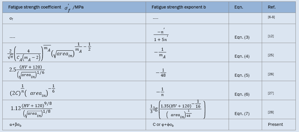
This is the well-known Basquin relation and has been still widely used even today, which indicates that it is very important to choose a suitable method of handling data. It is noted that there are some relations between the fatigue parameters (fatigue strength coefficients and exponents) of the S-N curves and mechanical properties [3-5] . For instance, the fatigue strength coefficient , refined as the true stress required to cause fracture in one reversal, equals to the stress intercept at 2Nf=1 and is chosen as the tensile strength or the true fracture strength . However, there are many different debates: the differences among σf, and σb sometimes are small [3]; to a good approximation, it is chosen for most materials [5-7] that equals to . The fatigue strength exponent b is defined as the power to which the life in reversal must be raised to be proportional to the stress amplitude and taken as the slope of the logarithm ordinate and abscissa. Moreover, different references reported different value ranges for b such as -0.125~-0.2 [8], -0.05~-0.12 [5,9], -0.05~-0.2 [3] and -0.05~-0.15 [6]. Morrow et al. [10] proposed a quantitative relation between b and cyclic strain hardening exponent n (Table 1) as follows
Table 1. Summary of the fatigue strength coefficients and exponents.
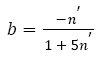 (3)
(3)
From representative data for different types of steels with n’<0.2, Ellyin [6] detected that eqn. (3) cannot predict b well, however, Landgraf [7] found that eqn. (3) can fit generally the experimental trend. In a word, the analysis results of fatigue curves mentioned above show that those existing functions predicting fatigue curves are phenomenological description related with the materials properties.
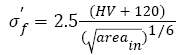
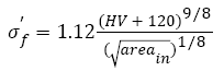
In recent years, the very high-cycle fatigue (>107 cycles, VHCF) behaviors of steels have arisen a great interest of many investigators. It was found that many factors such as inclusion size [11-13], sample surface treatment [14-18], experimental environment [16,19-21] and loading type [14,22] etc. can change the shape of S-N curve, and hence change the values of  and b. Especially, Akiniwa et al. [23], Chapetti et al. [24], Mayer et al. [25] and Liu et al. [26] developed some new quantitative expressions of and b in the VHCF regime as shown in Table 1 and the corresponding Basquin relations are as follows respectively:
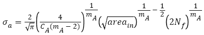 (4)
(4)
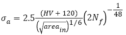 (5)
(5)
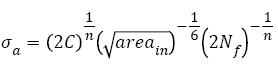 (6)
(6)
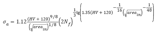 (7)
(7)
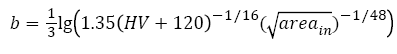
Here,  is the square root of inner inclusion area perpendicular to the applied stress axis (μm), HV is the Vickers hardness (kgfmm-2); mA (14.2, JIS SUJ2 [23]), CA (3.44 x 10⁻²¹, JIS SUJ2 [23]), C (6.47 x 1098, 100Cr6 [25]) and n (28.82, 100Cr6 [25]) are material constants.
It is shown that from eqns. (4)-(7) and Table 1 that the most fatigue str ength coef f icients  have r elations with inclusion size
  and two coefficients in eqns. (5) and (7) also have relations with HV; only one fatigue strength exponent b in eqn. (7) has relation with inclusion size
  and HV, the other exponents are constant. This arises two questions of great concern: 1) for the same material with almost the same size of inclusion and wide range of tensile strength, what on earth are the relations between tensile strength and parameters of S-N curves (
 and b)? 2) What is the fatigue mechanism determining and b? To find them, two typical high-strength steels with a wide range of tensile strength including AISI 4340 steel (tensile strengths ranged from 1300 MP to 2400 MPa) under push-pull load and SCM 435 steel (tensile strengths ranged from 990 MPa to 1900 MPa) under rotating-bending load were chosen to investigate the parameters of S-N curves.
Assortment and Definition of S-N Curve
The parameters of S-N curves can be obtained by eqns. (1) or (2). To compare and analyze easily, it is necessary to assort and define S-N curve of metallic materials. According to the shape, fatigue curves of steels can be divided into three types as schematically shown in Figure 1: I) continuous decreasing type, which can be subdivided into one linear (Figure 1a) or two-stage linear curves (Figure 1b); II) fatigue limit type ( Figure 1c), which will show a horizontal asymptotic tendency; III) step-wise [27,28] (duplex [29,30]) type (Figure 1d), which will show two knee points. S-N curves of most metallic materials can show Type I or II. For steel with the highest production and the widest usage among metallic materials, the three types of I [31-34], II [1,8,11,15] and III [27-30] can exist.

Figure 1: Schematic of the type of S-N curves: (a) and (b) Continuous decreasing; (c) Fatigue limit; (d) Duplex curve.
Existing results indicate that the shape of S-N curve relates with the cycles to failure, type of materials, even the number of tested samples and range of stress amplitude. It is well-known that there are some standards of the experimental planning of fatigue testing such as ISO 12107-2003. However, different investigators chose different cycles to terminate the fatigue tests, different number of tested samples and the levels of stress amplitudes. For example, 107, 108, 5 x 10⁸, 109, even 1010 can be chosen as the terminated cycles. An S-N curve has five fatigue data, however, the other has more than 100 data. The same S-N curve may be thought as continuous decreasing type by some people, however as duplex curve by others. Some materials show continuous decreasing type within 108 cycles but maybe show fatigue limit type beyond 1010 cycles. To normalize and simply compare, it is necessary to define the testing parameters that influence the shape of S-N curve.
In this paper, the terminated cycle is identical (VHCF: 109 cycles); in each group, the total number of tested samples is almost the same (not less than 20 or 10); the number of stress amplitude levels is almost the same (not less than 5); the maximum stress amplitude is not very high (not more than 1.5~2 times of fatigue strength). The S-N curve can be fitted as a line with the slope of nonzero, most data distribute within a certain error band (Figure 1a), this is a typical continuously decreasing type; besides, in its lower part, the S-N curve may be fitted as another line with the slope nonzero, this is also a continuous decreasing type (Figure 1b). In its lower part, the S-N curve seems to be as a horizontal asymptotic line and can be fitted as a line with the slope of near zero, which is defined as fatigue limit type (Figure 1c). Some parts of S-N curve can be fit as two lines with the slopes nonzero, the third as a line with the slope of near zero, which is defined as duplex curve (or step-wise curve) (Figure 1d).
Two typical steels were chosen to figure out the type of S-N curves and to study the relation between their types and corresponding fatigue mechanisms.
Analysis of S-N Curves of Steels with a Wide Strength Range
AISI 4340 steel with a wide strength range under push-pull loading: AISI4340 steel with a very wide range of tensile strength, one of the excellent quenched and tempered low-alloy steels [14,17,35-41], was chosen to study the relation between S-N curves and tensile strength. The ingredient of current AISI 4340 [42]. To obtain a wider range of strength, six heat-treatment procedures: heated to 850°C for 10 min and quenched in oil, did not temper and tempered at 180°C, 250°C and 350°C for 120 min and at 420°C, 500°C for 30 min respectively, were employed and the specimens were defined as A, B, C, D, E and F, correspondingly. The main microstructure of sample A is needle- or plate-shaped martensites; those of samples B-D are tempered martensites; those of samples E and F are tempered troostites, which was shown in detail [42]. The tensile strengths of samples A-F were listed in Table 2. The S-N features were analyzed by the widely used method of Basquin relation as following:
Table 2. The data of AISI 4340 steel and the parameters of Basquin relation for the very high-cycle fatigue S-N curves.
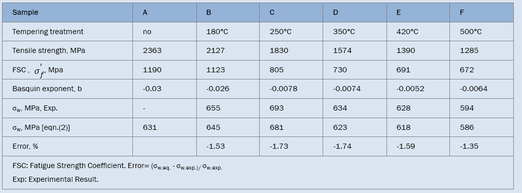
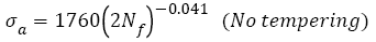
Figure 2 shows that the VHCF S-N curves of AISI 4340 treated by different tempering procedures were well fitted by eqn. (2) and their expressions are

Figure 2: Basquin relation fitting of VHCF S-N curves of AISI 4340 steel treated at different tempering temperatures. (a) untempered; (b) 180°C; (c) 250°C; (d) 350°C; (e) 420°C; (f) 500°C. (Data in (b)-(f) collected from ref. [42])
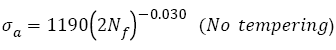 (8)
(8)
 (9)
(9)
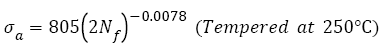 (10)
(10)
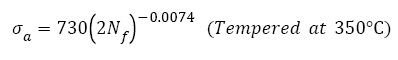 (11)
(11)
 (12)
(12)
 (13)
(13)
As shown in Figure 2, fatigue data of samples without tempering are within the 15% error band; however, others are within the 5% error band. This indicates that Basquin relation can express well the VHCF S-N curves of AISI 4340 steel tempered at different temperatures and those S-N curves show decreasing type, of which step-wise or duplex type reported [29,30,43,44] was not found. Murakami et al. [45,46] carried out push-pull tests using JIS-SCM435 and JIS-SUJ2 and also found the same results. The reason may be that for AISI 4340, the average diameter of the inclusion, which of samples A-F is 27, 28, 27, 32, and 41 μm respectively, is greater than 20 μm [11].
Eqns. (8)-(13) were plotted together in Figure 3 and the analysis data of corresponding equations were listed in Table 2, it can be seen that the fatigue strength exponents b of samples C to F are almost equal and their S-N curves are almost parallel. Their fatigue strengths at 109 cycles incr ease with incr easing the fatigue str ength coef f icients However, for samples A and B, the fatigue strength coefficients are higher and the fatigue strength exponents b are lower than the former (Figure 3), so that the stress amplitude of sample A is higher than that of sample B at lower cycles, the trend becomes reverse at higher cycles. It is noted that for samples F to C, the fatigue strengths at 109 cycles increase and then begin to decrease for samples B and A, the turning point appears at sample C which has the maximum fatigue strength.

Figure 3: Six VHCF S-N curves expressed by Basquin relation for AISI 4340 steel samples.
Figure 4 displays the relation between analysis results of S-N curves and tensile strength. In Figure 4a, with true tensile strength  increasing, fatigue strength (FS) coefficient
  under VHCF load increases linearly and the relation can be fitted as follows:
 (14)
(14)
The data are within the 15% error band, this illustrates that the relation between fatigue strength coefficient and true tensile strength is linear, which is different from the relation mentioned [5-7]  . It is also found in Figure 4b that there is a linear relation between true tensile strength and tensile strength, i.e.
 (15)
(15)
The data are within the 5% error band.
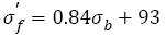
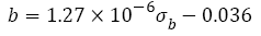
Combining eqn. (14) and eqn. (15), it can be deduced that the relation between fatigue strength coefficient  and tensile strength should be linear, as indicated in Figure 4c, the relation can be fitted as follows:
 (16)
(16)

Figure 4: S-N curve analysis of AISI 4340 steel by Basquin relation: (a) true tensile strength and fatigue strength (FS) coefficient; (b) tensile strength and true tensile strength; (c) tensile strength and fatigue strength (FS) coefficient; (d) tensile strength and Basquin exponent.
The error band is within 10%, this illustrates that the linear relation can well express the relation between fatigue strength coefficient and tensile strength  . The linear relation is more accurate than that reported [3]
  . Referring the fatigue strength coefficients
 listed in Table 1, it can be known that for a specific steel, the inclusion size can be considered as a constant, so that the fatigue strength coefficients
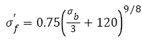
  in eqns. (4) and (6) are constants, which is obviously not in accordance with eqn. (16). However, the fatigue strength coefficients in eqns. (5) and (7) relate with HV, the coefficients respectively are
 (17)
(17)
 (18)
(18)
We chose the average inclusion size of 26 μm at fatigue origins (For present AISI 4340 specimens A-F, the inclusion sizes observed at fatigue origins are about 24-30 μm) and the relation between hardness HV and tensile strength is 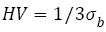 [47], eqns. (17) and (18) can be written to correspondingly:
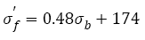 (19)
(19)
 (20)
(20)
Using software of Origin, in the strength range from 1200 MPa to 3000 MPa, eqn. (20) can be approximately rewritten as the linear relation
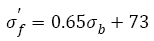 (21)
(21)
The change trend of eqn. (16) is similar with those of eqns. (19) and (21); however, the calculated results by eqns. (19) and (21) are obviously different with that by eqn. (16) because of the striking differences of slopes and intercepts. The reason may be that eqns. (19) and (20) mainly focus on the influence of inclusion and do not involve the change of tensile strength in a much wide range. However, eqns. (16), (19) and (21) confirm the truth that the linear relation between fatigue strength coefficient and tensile strength exists.
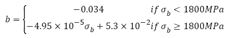
As shown in Figure 4d, the fatigue strength exponent b under VHCF load almost maintains constant (-0.0067) with tensile strengths increasing, however, when tensile strength is more than ~1800 MPa, fatigue strength exponent begins to decrease in a linear fashion. The relation can be written as
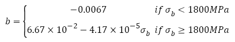 (22)
(22)
Most fatigue data in Figure 4d are within the 20% error band. In fact, when tensile strength is less than 1800 MPa, the relation between fatigue strength exponent and tensile strength can be fitted as a line
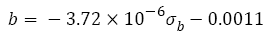 (23)
(23)
But it is worth noting that when the strength ranges from 1200 to 1800 MPa the slope (-3.72 x 10⁻⁶) in eqn. (23) is so small that the values of eqn. (23) (-0.0056 to -0.0078) are within the 20% error band shown in Figure 4d , therefore, it can be considered approximately as a constant (-0.0067).
Besides, the fatigue strength exponent b in eqn. (7) is
 (24)
(24)
By substituting average inclusion size 26 μm at fatigue origins and the relation between hardness HV and tensile strength mentioned above, eqn. (24) becomes to
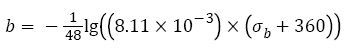 (25)
(25)
In the strength range from 1200 MPa to 2400 MPa, eqn. (25) can be approximately rewritten as the linear relation
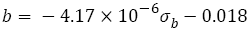 (26)
(26)
The values of b in eqn. (22) also are more than those in eqns. (25) or (26). This may be because S-N curve in VHCF regime becomes gradually varying, as shown schematically in Figure 1c. But it is worth noting that the slope (-4.17 x 10⁻⁶) in eqn. (26) is so small that the values of eqn. (26) are -0.023 to -0.028 when the strength are from 1200 MPa to 2400 MPa, hence it can be considered approximately as a constant (-0.026).
When σb<1800 MPa, the fatigue strength exponent b almost keeps unchanging and fatigue strength coefficient increases with tensile strength increasing so that fatigue strength increases with tensile strength; when σb ≥ 1800 MPa, the fatigue strength coefficient σf increases, however the fatigue strength exponent b substantially decreases with tensile strength increasing (Figure 4d) which leads to decreasing of fatigue strength. Therefore, maximum fatigue strength could exist at an adequate tensile strength. In addition, very high cycle fatigue strengths of samples B to F at 109 cycles can be calculated by eqns. (8)-(13), respectively. It can be concluded from Table 2 that the errors between calculated fatigue strength by Basquin relation and experimental value obtained by staircase method are less than 2%, which is quite satisfactory for fatigue testing. Compared with samples B-F, fatigue data of sample A were too scattered to obtain fatigue strength by staircase method.
In summary, it can be concluded that there are some quantitative relations between parameters of S-N curve (fatigue strength coefficient  and exponent b) and tensile strength (Table 1). By using those parameters changing tendency of S-N curves and fatigue strength can be predicted (Table 2).
SCM 435 steel with a wide strength range under rotating-bending loading: For AISI 4340 steel, the relations between the features of S-N curves and tensile strength with a wide range under push-pull loading were discussed. It is necessary to study those relations under rotating-bending loading, especially, step-wise or duplex type S-N curve [29,30,43,44] often appears under this condition. However, there are very rare fatigue data for a specific steel with a wide range of tensile strength, luckily, fatigue data of SCM435 steel with 5 different strength levels were found [48]. Five heat-treatment procedures: heated to 855°C for 30 min and quenched in oil, did not temper and tempered at 160°C, 300°C, 500°C and 600°C for 60 min were employed and the specimens were defined as A, B, C, D and E, respectively. The tensile strengths of samples A-E are 1898, 1785, 1734, 1303 and 991 MPa. The S-N curve features of SCM 435 steel were studied by the Basquin relation as below:
The VHCF S-N curves of SCM 435 steel treated by different tempering procedures were fitted by eqn. (2) and shown in Figure 5. Their fitting equations can be written as
 (27)
(27)
 (28)
(28)
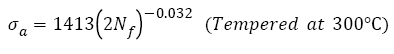 (29)
(29)
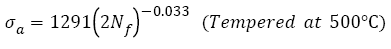 (30)
(30)
 (31)
(31)

Figure 5: Basquin relation fitting of S-N curves of SCM 435 steel after different tempering temperatures. (a) untempered; (b) 160°C; (c) 300°C; (d) 500°C; (e) 600°C; (f) summary graph of five S-N curves. (Data in (a)-(e) collected from ref. [48])
From Figure 5a-5e, it is found that fatigue data of all samples are within the 15% error band. This implicates that Basquin relation can describe well the S-N curves of SCM 435 steel tempered at different temperatures, and those S-N curves also show continuous decreasing type, similar to AISI 4340 steel, of which step-wise or duplex type reported [29,30,43,44] was also not found. However, S-N curves of samples A and B are considered as duplex type [48], this is because the number of stress amplitude levels [48] for samples A and B is more than that in present treatment.
Eqns. (27)-(31) were plotted together in Figure 5f, it can be found that the fatigue strength exponents b of samples B to E are almost equal and their S-N curves are almost parallel, their fatigue strengths at 109 cycles increase with increasing the fatigue strength coefficients σf. However, for samples A and B, the fatigue strength coefficients are higher and the fatigue strength exponents are lower than the former (Figure 5f), so that the stress amplitude of sample A is higher than that of sample B at lower cycles, their stress amplitudes are almost equal, even the former trend becomes reverse at more higher cycles. It is noted that for samples E to B, it is estimated fatigue strengths at 109 cycles increase and then begin to decrease for sample A, which indicates that a maximum fatigue strength exists.
Figure 6a and 6b show the parameters of S-N curves depending on the tensile strengths. The fatigue strength (FS) coefficient  under VHCF load almost increases linearly with tensile strength increasing and their relation can be expressed as below:
 (32)
(32)

Figure 6: S-N curve analysis of SCM 435 steel by Basquin relation: (a) fatigue strength coefficient and tensile strength (b) Basquin exponent and tensile strength.
From Figure 6, it is seen that the data are within the 10% error band, which indicates that the relation between fatigue strength coefficient and tensile strength is linear. Eqn. (32) is similar with eqn. (16) in the form. This implicates that if the steels with a wide range of tensile strength have the same type of continuous decreasing S-N curves, the fatigue strength coefficent  and tensile strength will show a linear relation.
Figure 6b shows the relation between fatigue strength exponent b and tensile strength. The fatigue strength exponent almost keeps unchanging (-0.034) as tensile strength increases; when tensile strength is more than ~1800 MPa, fatigue strength exponent begins to decrease in a linear fashion. The relation can be written as
 (33)
(33)
From Figure 6b, it is seen that all the fatigue strength exponents are within the 5% error band. In fact, when tensile strength is less than 1800 MPa, the relation between fatigue strength exponent and tensile strength can also be fitted as a line
 (34)
(34)
But it is worth noting that when the strength range from 1200 MPa to 1800 MPa the slope (1.27 x 10⁻⁶) in eqn. (34) is so small that the values of eqn. (34) (-0.0345 to -0.0337) are within the 2% error band, therefore, it can be considered approximately as a constant (-0.034).
When terminated cycle equals to 109, fatigue strengths of samples A-E calculated by eqns. (27)-(31) are 737 MPa, 743 MPa, 691 MPa, 621 MPa and 420 MPa, respectively. Obviously, the calculated fatigue strengths of samples C-E are slight smaller than those estimated from Figure 5c-5e. This indicates that to obtain the more precise fatigue strength needs more enough broken and suspended fatigue samples in VHCF regime. It should be noted that in Figures 2 and 5 there are some selected data without rigor (suspended samples) because of limited samples.
In a word, it can be found that there are also some quantitative relations between the parameters (fatigue strength coefficient σf and exponent ) of S-N curve and tensile strength. By using those parameters, changing tendency of S-N curves and fatigue strength can be obtained.
Summary of the Relations between S-N Curve Features and Tensile Strength as well as their Application in Material Design
The relations between S-N curve features and tensile strengths of AISI 4340 steel and SCM 435 steel were studied as above and some results can be summarized as below:
1) Fatigue strength coefficients of AISI 4340 steel and SCM 435 steel almost increase linearly with tensile strengths increasing and eqns. (16), (19), (21) and (26) can be unified as the form i.e.
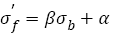 (35)
(35)
Where, α and β are constants related with materials.
2) For AISI 4340 steel and SCM 435 steel, if tensile strengths are less than a specific tensile strength  (say ~ 1800 MPa), fatigue strength exponents almost keep as a constant C (-0.0067 or -0.034) with tensile strengths increasing; if tensile strength is more than
  , fatigue strength exponents linearly decreases with tensile strengths increasing, the eqns. (22) and (33) can be written as the general form:
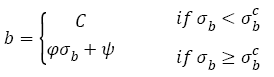 (36)
(36)
Where, φ and ψ are constants related with materials.
But it is worth noting that all S-N curves of AISI 4340 and SCM 435 are continuous decreasing type (Figures 2 and 5). It can be deduced that if the types of S-N curves are not the same, eqns. (35) and (36) may be not necessarily suitable.
By analyzing fatigue strength exponent and coefficient and related fatigue data mentioned earlier, we can find three possible methods to improve fatigue strength as shown in Figure 7: (1) Fatigue strength coefficient keeps constant and fatigue strength exponent b increases ( Figure 7 S-N curve 1). At this case, the higher fatigue strength exponent, the higher fatigue strength. (2) Fatigue strength exponent b keeps constant and fatigue strength coefficient ÃÆïÃâÿÃâýÃÆïÃâÿÃâý ′ increases ( Figure 7 S-N curve 2). At this case, the higher fatigue strength coefficients, the higher fatigue strength; (3) Both fatigue strength coefficient  and fatigue strength exponent b increase (Figure 7 S-N curve 3). To enhance the fatigue strength of metallic materials by modifying those parameters will be presented in coming paper.
The Mechanisms for Influencing the S-N Curves Parameters related with Tensile Strengths
In section above, the general relations between the parameters of S-N curves and tensile strengths are summarized. The mechanisms under laid the relations are investigated in this section.
A perfect material loaded under the stress amplitude of fatigue strength coefficient (σf) will suspend to 109 cycles, this is to say that S-N curve should be a level line and  can be named as an ideal fatigue strength (Figure 7). However, a real material after alternating load will yield some local damages because of various defects (point defects, dislocations, boundaries, inclusion and so on), this makes S-N curve not a level but different types shown schematically in Figures 1 and 7. Therefore, fatigue strength exponent b can be named as fatigue damage exponent. Combining previous results, the mechanisms controlling fatigue strength exponent related with tensile strength are discussed as follows.

Figure 7: Schematic illustration of improving fatigue strength (FS) by adjusting fatigue strength coefficient and fatigue strength exponent.
The Relation between Fatigue Strength Coefficient and Tensile Strength
From Basquin relation eqn. (2), one can see that the fatigue strength coefficient should equal to the true stress required to cause fracture in one reversal cycle, namely, ideal fatigue strength. In fact, fatigue testing results of real materials can be influenced by many factors such as loading mode, loading frequency, number of tested samples, range of stress amplitude and so on. So the fatigue strength coefficient almost impossibly equals to the true fracture stress, but it should relate with strengthening mechanism such as precipitate strengthening and so on, which determine the stress amplitude to sustain in one reversal. In a word, it is apparent that the fatigue strength coefficient and tensile strength exit a linear relation.
The Relation between Fatigue Strength Exponent and Tensile Strength
As mentioned above, fatigue strength exponent b represents fatigue damage degree in the course of cyclic loading. For very high-cycle fatigue, a very large fraction of life is spent in crack initiation, therefore, b will have an obvious relation with fatigue crack initiation. For fatigue crack origins, there are some typical cases such as surface scratch (Figure 8a) and inner inclusion (Figure 8b). The granular bright facet (GBF) [18,30] area around inclusion can be observed in Figure 8b, however, no GBF area can be observed in Figure 8a because of crack initiation at a surface scratch. As shown in Figure 9a, for AISI 4340 steel, when tensile strength is in the range from 1200 to 2000 MPa, the ratio of inner cracking sites (RICS, the ratio of the number of failure samples originated from the inner inclusion site to the total number of failure samples) gradually increases with tensile strength increasing, and fatigue cracks appear both on the surface and in the interior for samples C to F, which implies that the there is a major fatigue mechanism in this tensile strength range, correspondingly, fatigue strength exponent b almost keeps constant; When tensile strength is more than 2000 MPa, all fatigue cracks originate from inner inclusions, therefore the ratios of inner cracking sites for samples A and B are 100%, which indicates that fatigue mechanism in this tensile strength range changes, at the same time, fatigue strength exponent begins to decrease linearly.

Figure 8: Two fatigue crack origin of fatigue samples for AISI 4340 steel: (a) surface (Sample F tempered at 500°C, σa=600 MPa, Nf=5.31 x 10⁵ cycles); (b) inner inclusion (Sample C tempered at 250°C, σa=660 MPa, Nf =4.43 x 10⁶ cycles).

Figure 9: The relation between the ratio of fatigue crack initiation sites and fatigue strength exponent of steels with tensile strength increasing: (a) AISI 4340; (b) SCM 435.
For SCM 435 steel, similar results can be observed. When tensile strength is in the range from 900 to 1700 MPa, the ratio of surface cracking sites (RSCS, the ratio of the number of failure samples originated from the surface site to the total number of failure samples) equals 100%, namely, all fatigue cracks originate from surface, which implies that the fatigue mechanism is the same one in this tensile strength range, correspondingly, fatigue strength exponent b almost keeps constant; when tensile strength is more than 1700 MPa, RSCS of sample A is 64%, which indicates that fatigue mechanism changes, at the same time the fatigue strength exponent begins to decrease linearly as shown in Figure 9b.
In a word, the changing of fatigue cracking sites leads to the variation tendency of fatigue strength exponent. In addition, there are some changes in microstructure and fractographs of AISI 4340 steel tempered at different temperatures. The corresponding mechanism can be roughly explained as following:
Untempered sample A has the indistinct dividing line between crack growth area and final fracture area and flat fracture surface (Figure 10a); samples C-F tempered at 180, 250 350, 420 and 500°C have the obvious dividing lines and growth ridges (Figure 10b-10f), especially sample C shows some regular fan shaped zones as shown in Figure 10c. This implicates that their plastic deformation abilities are different. The reason maybe that sample A with full martensite microstructure has so many defects such as supersaturated interstitial carbon atoms, high density dislocations [49,50], subgrain boundaries and so on that the ability of plastic deformation is very weak and the tensile strength is very high; at this case, the fatigue sensitivity to defects is much higher [42] and fatigue damage degree in the cause of fatigue crack initiation becomes very high, therefore sample A has the lowest fatigue strength exponent b (Figure 9a).

Figure 10: The macroscopic morphologies of fatigue samples for AISI 4340 steel processed at different tempering temperatures: (a) untempered (σa=680 MPa, Nf =4.34 x 10⁷ cycles); (b) 180°C (σa=750 MPa, Nf =2.05 x 10⁷ cycles); (c) 250°C (σa=660 MPa, Nf =4.43 x 10⁶ cycles); (d) 350°C (σa=650 MPa, Nf =4.72 x 10⁶ cycles); (e) 420°C (σa =640 MPa, Nf =4. 23 x 106 cycles); (f) 500°C (σa=620 MPa, Nf =9.14 x 10⁵ cycles).
Martensite gradually decomposes with tempered temperature increasing (150~350°C). Compared with sample A, sample B with tempered martensite has less defects, smaller tensile strength and higher plastic deformation, which lead to the formation of obvious dividing lines and growth ridges (Figure 10b-10f); at this time, the fatigue sensitivity to defects is lower [42] and fatigue damage degree decreases, therefore fatigue strength exponent b increases (; sample C with the microstructure of decomposed martensite and rod shaped carbides has no much high tensile sFigure 9atrength, but better plastic deformation and lower fatigue sensitivity, distinct regular fan shaped zones and higher fatigue strength exponent b.
When tempered temperature reaches 250~400°C, the decomposition of martensite is essentially over, typical tempered martensite in sample D tempered 350°C forms; when tempered temperature is over 400°C, cementite appears and gradually grows with tempered temperature increasing and the microstructures of the samples E and F, respectively tempered at 420 and 500°C, are tempered troostites. For samples D-E, tensile strengths are not high, hence the plastic deformation ability is better, fatigue sensitivity is lower, and fatigue damage degree is not high, finally, their fatigue strength exponents keep unchanging.
In summary, for AISI 4340 steel treated by different heat treatment procedures, fatigue strength exponent firstly keeps constant and then deceases obviously with tensile strength increasing as shown in Figure 9a. The above mechanisms to control parameters of S-N curves may hint that enhancing the fatigue strength coefficient by using adequate strengthening mechanisms and/or lowering fatigue strength exponent by decreasing harmful defects can improve the fatigue strength of the steels.
The S-N curves of typical high strength steels such as AISI 4340 and SCM 435 were investigated by using Basquin relation.
The changes of fatigue strength coefficient  and exponent b lead to the corresponding changes of S-N curves. If the steels have a wide range of tensile strength and the S-N curves have continuous decreasing type, the relation between fatigue strength coefficient and tensile strength is linear, i.e.
 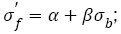 the relation between fatigue strength exponent and tensile strength almost shows a horizontal line within certain range of tensile strength and then declines and becomes linear as b=φ+ÃÆÃÂÃâââ¬Â¢σ . Basic fatigue mechanisms controlling S-N curve parameters with increasing tensile strength were briefly investigated. Fatigue strength coefficient
  relates with strengthening mechanisms of materials.The change of fatigue cracking sites, the variations of microstructures and fatigue fractographys of steels treated by different heat treatments lead to the change of fatigue strength exponent b with tensile strength increasing.
This work is supported by National Natural Science Foundation of China (NSFC) under Grant Nos. 51301179, 51331007. Dr. Pang JC would like to thank Prof. Sakai T for sending the important reference.