International Journal of Innovative Research in Computer and Communication Engineering
ISSN ONLINE(2320-9801) PRINT (2320-9798)
ISSN ONLINE(2320-9801) PRINT (2320-9798)
Gobu.CK1 and Priya.R2
|
| Related article at Pubmed, Scholar Google |
Visit for more related articles at International Journal of Innovative Research in Computer and Communication Engineering
In the process of signal acquisition and transmission image signals might be corrupted by impulse noise. Efficient VLSI implementation is presented in this paper, in order to remove impulse noise. In order to perform better visual quality, edge features should be preserved. Pixels that are detected as noisy are filtered, the others remain unchanged. Here fixed value impulse noise is removed and implemented in VLSI. The VLSI architecture of our design yields a processing rate of about 200 MHz by using TSMC 0.18μm technology. Compared with the state-of-the-art techniques, this work can reduce memory storage by more than 99%. The design requires only low computational complexity and two line memory buffers. Its hardware cost is low and suitable to be applied to many real-time applications.
KEYWORDS |
| Image denoising, impulse noise, impulse detector, architecture |
I. INTRODUCTION |
| Image processing is widely used in many fields, such as medical imaging, scanning techniques, printing skills, license plate recognition, face recognition, and so on. In general, images are often corrupted by impulse noise in the procedures of image acquisition and transmission. The noise may seriously affect the performance of image processing techniques. Hence, an efficient denoising technique becomes a very important issue in image processing. According to the distribution of noisy pixel values, impulse noise can be classified into two categories: fixed-valued impulse noise and random-valued impulse noise. Impulse noise is also known as salt-and-pepper noise because the pixel value of a noisy pixel is either minimum or maximum value in grayscale images. We only focus on removing the random-valued impulse noise from the corrupted image in this paper. |
II. THE PROPOSED DTBDM |
| The noise considered in this paper is random-valued impulse noise with uniform distribution as practiced in Here, we adopt a 3 3 mask for image denoising. Assume the pixel to be denoised is located at coordinate and denoted as pi,j, and its luminance value is named as fi,j, as shown in |
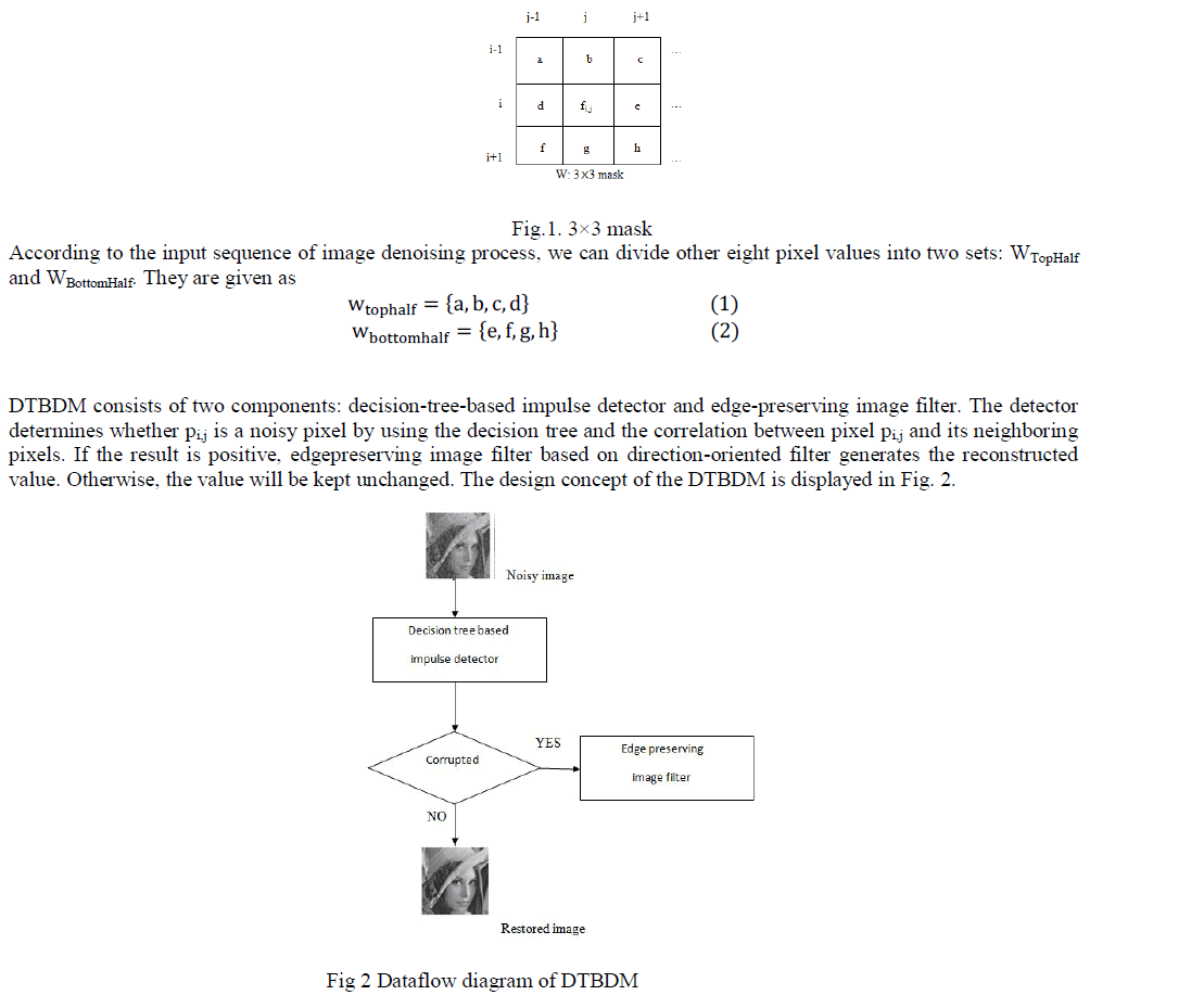 |
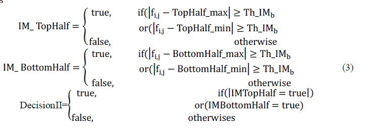
| DECISION TREE BASED IMPULSE DETECTOR |
| In order to determine whether pi,j is a noisy pixel, the correlations between pi,j and its neighboring pixels are considered . Surveying these methods, we can simply classify them into several ways—observing the degree of isolation at current pixel , determining whether the current pixel is on a fringe or comparing the similarity between current pixel and its neighboring pixels Therefore, in our decision-tree-based impulse detector, we design three modules—isolation module (IM), fringe module (FM), and similarity module (SM). Three concatenating decisions of these modules build a decision tree. The decision tree is a binary tree and can determine the status of pi,j by using the different equations in different modules. First, we use isolation module to decide whether the pixel value is in a smooth region. If the result is negative, we conclude that the current pixel belongs to noisy free. Otherwise, if the result is positive, it means that the current pixel might be a noisy pixel or just situated on an edge. The fringe module is used to confirm the result. If the current pixel is situated on an edge, the result of fringe module will be negative (noisy free); otherwise, the result will be positive. If isolation module and fringe module cannot determine whether current pixel belongs to noisy free, the similarity module is used to decide the result. It compares the similarity between current pixel and its neighboring pixels. If the result is positive, pi,j is a noisy pixel; otherwise, it is noise free. The following sections describe the three modules in detail. |
| ISOLATION MODULE |
| The pixels with shadow suffering from noise have low similarity with the neighboring pixels and the so-called isolation point. The difference between it and its neighboring pixel value is large. According to the above concepts, we first detect the maximum and minimum luminance values in WTopHalf, named as TopHalf_max, TopHalf_min, and calculate the difference between them, named as TopHalf_diff. For WBottomHalf , we apply the same idea to obtain BottomHalf_diff. The two difference values are compared with a threshold Th_IMa to decide whether the surrounding region belongs to a smooth area. The equations are as |
 |
| FRINGE MODULE |
| How to conclude that a pixel is noisy or situated on an edge is difficult. In order to deal with this case, we define four directions, from E1 to E4, as shown in Fig. 7. |
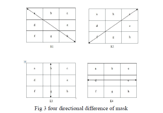 |
| We take direction E1 for example. By calculating the absolute difference between fi,j and the other two pixel values along the same direction, respectively, we can determine whether there is an edge or not. The detailed equations are as |
 |
III. SIMILARITY MODULE |
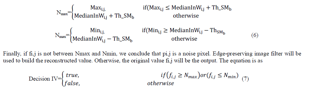
| The last module is similarity module. The luminance values in mask W located in a noisy-free area might be close. The median is always located in the center of the variational series, while the impulse is usually located near one of its ends. Hence, if there are extreme big or small values, that implies the possibility of noisy signals. According to this concept, we sort nine values in ascending order and obtain the fourth, fifth, and sixth values which are close to the median in mask W. The fourth, fifth, and sixth values are represented as 4thinWi,j, MedianInWi,j, and 6thinWi,j. We define Maxi,j and Mini,j as |
| Maxi,j=6thinWi,j+ThSMa |
| Mini,j=4thinWi,j-ThSMa (5) |
| Maxi,j and Mini,j are used to determine the status of pixel pi,j. However, in order to make the decision more precisely,we do some modifications as |
 |
| Obviously, the threshold affects the quality of denoised images of the proposed method. A more appropriate threshold contributes to achieve a better detection result. However, it is not easy to derive an optimal threshold through analytic formulation.The fixed values of thresholds make our algorithm simple and suitable for hardware implementation. According to our extensive experimental results, the thresholds Th IMa, TH IMb, Th FMa, Th FMb, Th SMa, and Th SMb are all predefined values and set as 20, 25, 40, 80, 15, and 60, respectively. |
| EDGE-PRESERVING IMAGE FILTER |
| To locate the edge existing in the current W, a simple edge preserving technique which can be realized easily with VLSI circuit is adopted. Only those composed of noise-free pixels are taken into account to avoid possible misdetection. Directions passing through the suspected pixels are discarded to reduce misdetection. Therefore, we use Maxi,j and Mini,j, defined in similarity module, to determine whether the values of d, e, f, g, and h are likely corrupted, respectively. If the pixel is likely being corrupted by noise, we don’t consider the direction including the suspected pixel. In the second block, if d, e, f, g, and h are all suspected to be noisy pixels, and no edge can be processed, so fi,j estimated value of pi,j is equal to the weighted average of luminance values of three previously denoised pixels and calculated as (a+ b× 2+ c)/ 2.In other conditions, the edge filter calculates the directional differences of the chosen directions and locates the smallest one Dmin among them in the third block. The equations are as follows: |
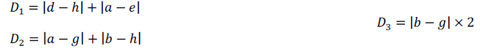 |
 |
| In the last block of Fig. 8, the smallest directional difference implies that it has the strongest spatial relation with pi,j and probably there exists an edge in its direction. Hence, the mean of luminance values of the pixels which possess the smallest directional difference is treated as fi,j. After fi,j is determined, a tuning skill is used to filter the bias edge. If fi,j obtain the correct edge, it will situate at the median of b,d, e, and g because of the spatial relation and the characteristic of edge preserving. Otherwise, the values of fi,j will be replaced by the median of four neighboring pixels (b, d, e, and g). We can express fi,j as |
| Fi,j=Median(fi,j,b,d,e,g) (9) |
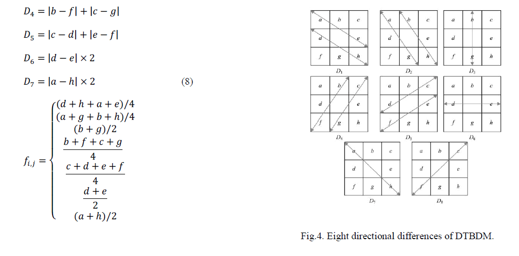
IV. VLSI IMPLEMENTATION OF DTBDM |
| DTBDM has low computational complexity and requires only two line buffers instead of full images, so its cost of VLSI implementation is low. For better timing performance, we adopt the pipelined architecture to produce an output at every clock cycle. In our implementation, the SRAM used to store the image luminance values is generated with the 0:18 μm TSMC/Artisan memory compiler and each of them is 512 × 8 bits. According to the simulation results obtained from Design Ware of SYNOPSYS we find that the access time for SRAM is about 5 ns. Hence, we adopt the 7-stage pipelined architecture for DTBDM. |
 |
V. CONCLUSIONS |
| A low-cost VLSI architecture for efficient removal of random-valued impulse noise is proposed in this paper. The approach uses the decision-tree-based detector to detect the noisy pixel and employs an effective design to locate the edge. With adaptive skill, the quality of the reconstructed images is notable improved. Our extensive experimental results demonstrate that the performance of our proposed technique is better than the previous lower complexity methods and is comparable to the higher complexity methods in terms of both quantitative evaluation and visual quality. The VLSI architecture of our design yields a processing rate of about 200 MHz by using TSMC 0:18 μm technology. It requires only low computational complexity and two line memory buffers. Therefore, it is very suitable to be applied to many real-time applications. |
References |
|