ISSN ONLINE(2278-8875) PRINT (2320-3765)
ISSN ONLINE(2278-8875) PRINT (2320-3765)
Samir Ghouali1, Mohammed Feham2, Yassine Zakarya Ghouali3
|
| Related article at Pubmed, Scholar Google |
Visit for more related articles at International Journal of Advanced Research in Electrical, Electronics and Instrumentation Engineering
Panel Co-integration is one of the most popular methods to reveal and evaluate the influence and the interactions that may exist between long-term variables; Co-integration is used in different field and enjoying unprecedented popularity due reliability, clarity and robustness. In this article, we conducted an investigation using very powerful mathematical model to verify if a long-term relationship exists between Cardiorespiratory hemodynamic signals, the methodology we applied in this paper is mainly based on four basic parts, in first part we applied unit root tests to assess the stationarity of series, the second step is to apply the test of Co-integration model and quantify this long-term relationship. Finally we applied the Granger causality tests to the entire panel that consists of 186 patients taken from Montreal Hospital / General MF (Massachusetts General Hospital / Marquette Foundation) database. The results found in this study show the long-term interaction between the Cardiorespiratory hemodynamic signals, and reveals how the understanding of these interactions can help the doctors to understand the risks that may exist between these interactions. The originality of this article is the number of variables incorporated in our model study. Unlike the majority of studies that are conducted with only two variables, our study is specified by its multidimensionality. The main advantage of a multidimensional and multivariate model is to solve a multitude of problemsthatprevent doctors to treat the patients betterandis not the case for studies in two dimensions.
Keywords |
| Panel Co-integration, Long-term, Panel Granger Causality,CardiorespiratoryHemodynamic signals, Multivariate study, (MGH / MF) waveform database. |
INTRODUCTION |
| Cardiovascular diseases are the leading cause of worldwide mortality, each year more and more people die cause the cardiovascular disease comparatively to any other causes, the number of deaths because the cardiovascular disease is estimated at 17.3 million and represent 30% of the total global mortality[1], among these deaths, 7.3 million were caused by coronary heart disease and 6.2 million by AVC (2008 statistics) [2].Over 80% of deaths happen in countries with low and middle income and occur almost equally between men and women.By 2030, almost 23.3 million people will die from cardiovascular disease (mainly heart disease and AVC), according to projections, these diseases should remain the leading causes of death [1, 3]. |
| However, the good fact is that 80% of premature heart attacks and AVC are avoidable. The detection of abrupt changes of blood pressure in real time, the potential heart attack prediction and providing the doctor a comprehensive state range of the patient are the keys of prevention. For a lighter treatment and better chances of recovery, early diagnosis is a real boon for patients suffering of cardiovascular diseases. The benefit of early diagnosis is that we can detect and make decisions to mitigate the risks of cardio-vascular problems. Two effective tools enable better diagnosis being early; the first way is to develop telemedicine applications that allow a real-time monitoring of the health status of the patient. The second procedure that will be complementary to the first is to make a mathematical model of a set of physiological data to help us better understand the phenomenon, assimilate and explain the temporal behavior of the studied physiological variables. |
| Our study will be based on this idea, have the necessary patient data in a critical condition in real time via a mobile smartphone. For this reason, a perfect analysis of the physiological data is necessary for us, the analysis is performed in two dimensions, the first is the most known, consists to use the theories of information and the processing algorithms signals to take and evaluate physiological parameters, our second aspect, called the second dimension of the examination is to find causality in long term (Co-integration) between physiological signals, it helps doctors and health officials to take all precautions to facilitate the choice of an appropriate intervention and decisions necessary for one unique goal, saving people's lives.One of the main reasons behind the application of Co-integration and causality in panel data is to obtain statistical power to improve the interpretation of results. Unfortunately, tests of Co-integration and causality using a panel data involve several complications; first of all, the panel data usually have a large amount of heterogeneity which makes the parameters difficult to model. Secondary, when an empirical study has alarge number of data in two dimensions, as our study, a major challenge appears during the computer implementation. |
| Several methods exist in this context, beginning with the methods of causality, the first causality was proposed andintroduced by Wiener and Granger (Nobel prize 2003) and become a fundamental theory for the analysis of dynamic relationships between the time series, Sims has presented a slightly different specification test, considering that if future values y help explain the present values of y then y is the cause ofy. |
LITERATURE REVIEW |
| Numerous studies in recent years have been devoted to the evaluation of causality; several applications of the latter are omnipresent in areas ranging from the economy [4, 5], climatology [6, 7, 8], society [9], directed information theory in networks [10], psychiatry [11], brain imaging field [12], ophthalmology [13], genetics [14] and especially the analysis of biological systems, with a very special emphasis on the neural field [15,16,17,18,19,20,21,22,23,24,25,26], the study of cardiac signals [27,28,29,30,31,32,33,34,35] and cardiorespiratory [33,36] interactions.In the remainder of this article, we will look at studied panel data causality and panel Co-integration of a number of physiological signals, derived from the MGH / MF database,the approach was then applied to three leads ECG, ART (Arterial Pressure), PAP (pulmonary arterial pressure), CVP (Central Venous Pressure), RESP (Respiratory Impedance) and CO2, taken from the MGH / MF (Massachusetts General Hospital / Foundation Marquette) database, These signals are ideal for understanding causality. |
| Recent advances in mathematical modeling have great enthusiasm of researchers especially in analysis using panel data. The application of Co-integration and causality allows us to ask an important question, are the blood pressure, central venous pressure, pulmonary arterial pressure, respiration, and CO2 that outweighs the three ECG leads or the three leads ECG to a change in the hemodynamic respiratory variables? |
| The goal of the paper is to propose to study the direction of causality between the signals mentioned previously and test of Co-integration, our contribution in this article is based on the following points: |
| Three-dimensional analysis of the heart |
| Check if there is a long-term relationship between the three lead ECG and hemodynamic respiratory signals based on the panel Co-integration. |
| Modelize, and even quantify the rate of convergence of this long-term relationship if it exists. |
| Define the direction of causality between the three lead ECG and hemodynamic respiratory signals based on the panel Granger causality. |
| Try to understand the impact of hemodynamic respiratory signals on three leads ECG in the long-term. |
| The remainder of this paper is organized as follows: In Section 3, we give some definition of the variables. In Section 4, we will establish the data used and the methodology to follow. Then, in section 5 we present the test for nonstationarity. In section 6 we present the unit root tests. In section 7, 8, 9, and 10 we put in evidence the approach of Cointegration, the estimated long-term relationship and granger causality test respectively. Finally, we lead an analysis, scientific discussion, conclusion and a projection of perspectives. |
DEFINITIONS OF SOME VARIABLES STUDIED |
| ECG leads:Lead systems allow you to look at the heart from different angles. Each different angle is called a lead. The different leads can be compared to radiographs taken from different angles. |
| ART: Blood pressure is the pressure of blood in the arteries, also referred to as blood pressure because this pressure is the force exerted by the blood against the walls of arteries, tends the wall of the artery. |
| CVP: Central venous pressure (CVP) also known as: right atrial pressure (RAP) describes the pressure of blood in the thoracic vena cava near the right atrium of the heart; it reflects the amount of blood returning to heart and the heart's ability to pump blood into the arterial system. |
| PAP: Pulmonary arterial pressure measures the pressure in the pulmonary arteries, the latter carries blood from the right side of the heart to the lungs. |
DATA AND METHODOLOGY |
A. Data Analysis |
| The Massachusetts General Hospital / Marquette Foundation (MGH / MF) Waveform database is a comprehensive collection of electronic records hemodynamic and electrocardiographic signals stable and unstable patients in intensive care units, operating rooms and Cath labs heart. It is the result of collaboration between physicians, biomedical engineers and nurses of the Massachusetts General Hospital, which includes three ECG leads, arterial pressure, pulmonary arterial pressure, central venous pressure, respiratory impedance and CO2. This multi-dimensional cardiac data collected from various parts of body can effectively imitate the signals from various on body sensor nodes. |
| The original dataset contains total 250 sets of cardiac signals; each containing 12 to 86 minutes in most cases are about an hour of recording. we selected 186 people on 250 for our simulation, the latter contains all the signals mentioned previously against by the rest do not have the typical data for our studies, These signals include cardiac events such as premature ventricular contraction, supraventricular premature, tachycardia, bradycardia, ventricular pacing and ectopic beat, which are all manually annotated by clinical professionals. |
B. Methodology |
| In the analysis of the relationship in long-term of the data panel, the choice of the appropriate technique is an important theoretical and empirical question. Co-integration is the most appropriate technique to study the long-term relationship between our cardiorespiratory hemodynamics variables. The empirical strategy used in this paper can be divided into four main stages. First, unit root tests in panel series are undertaken. Second, if they are integrated of the same order, the Co-integration tests are used. Third, if the series are co-integrated, the vector of Co-integration in the long-term is estimated using the methods (FMOLS) and (DOLS). Finally, the Granger causality test in panel will be undertaken. |
NO-STATIONARITY OF THE SERIES: DETECTION TESTS |
A. Definition of non-stationarity |
| Most of the time series are non-stationary, ie the process that describes not verify at least one of the definition conditions of a stationary process given by: |
| 1. E(Yt) =μ ∀ t (Constant, not dependent on t). |
 |
WHY TEST THE PANEL UNIT ROOT? |
| The unit root tests administered to the panel data have several advantages over those time-series. First, the number of data used is more important because of the meeting of the individual dimension and the temporal dimension. |
| The Extending of the database has real interest, as it strengthens the power of unit root tests to distinguish the stationary or non-stationary series. Several studies show that the unit root tests on panel data are more powerful than those carried out on time series.Technical panel data may also be preferred because of their low restrictions; in fact, they capture effects specific to each patients, heterogeneity of the direction and magnitude of the parameters through the panel. In addition, these techniques allow the model to be selected with a high degree of flexibility by providing a relatively wide range of different specifications, from models with constant and deterministic trend up to models with no constant and no trend; within each model, there is the possibility of testing for common time effects. |
| Panel unit root tests are used to examine the degree of integration between ECG and our hemodynamic respiratory signs. To assess the stationary properties of the used variables, this study use five different panel unit root tests including Levin, Lin and Chu [37](herein referred to as LLC); Im, Pesaran, and Shin [38](hereinreferred to as IPS); Maddala and Wu [39], Breitung [40] (herein referred to as BRT) and Hadri[41]. For each technique, we test for unit roots in the panel using two types of models. The first model has a constant and a deterministic trend and the second model has only a constant and no trend.LLC and IPS seem to be the most use tests; LLC [37] is the procedure most commonly used. It is based on the ADF test, assumes a homogenous group.Levin et al [37] is based on the following equation: |
| Where z is the deterministic component and uis the stationary process. zcan be a fixed effect or time trend as well as a constant like zero and 1. The LLC test assumes that residuals are independently and identically distributed with mean zero and variance σ and ρ=ρ for all values of i. The coefficient of the lagged dependent variable is assumed to be homogeneous in all units of the cross section of the panel. The null hypothesis can be constructed as H: ρ = 1 which meansthat all series in the panel have a unit root whereas in the alternative hypothesis H: ρ < 1 which means that all series are stationary. |
| Im et al [38]; The IPS test is an extension of the LLC test that relaxes the homogeneous assumptions by allowing for heterogeneity in the autoregressive coefficients for all panel members. The basic equation for the panel unit root tests for IPS is as follows: |
 |
| Where y. stands for each variable under consideration in our model, ais the individual fixed effect, ε. are assumed to be independently and normally distributed random variables for all i and t with zero means and finite heterogeneous variance σ ïÿýïÿý. P is selected to make the residuals uncorrelated over time. The null hypothesis is that ρ = 0 for all i versus the alternative hypothesis that ρ < 0 for some i = 1,…,N and ρ = 0 for i = N +1,…, N. The IPS statistic is based on averaging individual Augmented Dickey-Fuller (ADF, hereinafter) statistics and can be written as follows: |
 |
| Where tis the ADF t-statistic for patient i based on the patient specific ADF regression, as in Eq. (2) IPS show that under the null hypothesis of non-stationary in panel data framework, the tÃÅÃ⦠statistic follows the standard normal distribution asymptotically. The standardised statistic tis expressed as: |
 |
| Maddala and Wu [39] propose a non-parametric and exact test which is based on Fisher (1932) test, and combining the P-values from individual unit root tests. This test is superior compared to the IPS test (Maddala and Wu, [39]; Maddala et al., 1997). Its advantage is that its value does not depend on different lag lengths -in the individual ADF regressions. Breitung [40], several studies have shown using a Monte Carlo simulation, as proposed by Breitung for unit roots in panel test is much more powerful than the LLC and IPS tests. LLC and IPS suffer from loss of power if individualspecific trends are included. This is due to bias correction, which also eliminates the average local alternative sequence. Breitung suggests a test statistic that does not use a bias correction whose power is significantly higher than the LLC or IPS tests.Hadri (2000); The Hadri-test is a residual-based Lagrange Multiplier (LM) test where the null hypothesis is that there is no unit root in any of the series in the panel against the alternative of a unit root in the panel. |
CO-INTEGRATION APPROACH |
| The concept of Co-integration can be defined as a systematic co-movement between two or more variables in the longterm. According to Engle and Granger [4], if X and Y are both non-stationary, one would expect that a linear combination of X and Y would be a random walk. However, the two variables may have the property that a particular combination of them Z = X − bY is stationary. If such a property holds true, we say thatX andY are Co-integrated. |
A. Panel Co-integration |
| It is now recognized in the scientific literature that the best methods for testing unit roots and Co-integration is to use methods based on a panel. These methods greatly increase the power of the tests and often involve a two-steps procedure. The first step is to test the panel unit root; the second is the panel Co-integration tests.For the 186 patients in our empirical study, heterogeneity may arise due to differences in sex, age of patients and many other things. To ensure wide applicability of any panel Co-integrationtest, it is important to take into account as much as possible heterogeneity between the different group members.Pedroni [42, 43, 44]developed a method based on panel Co-integration residues that can take into account the heterogeneity in individual effects, the slope coefficients and individual linear trends between patients. Pedroni[44], considers the following type of regression: |
| For a time series panel of observables y and Zfor members i = 1,…, N over time periods t = 1,…T. the variablesy and X are assumed to be integrated of order one, denoted I(1). The parametersaand δ allow for the possibility of individual effects and individual linear trends, respectively. The slope coefficients β are also permitted to vary by individual, so in general the Co-integrating vectors may be heterogeneous across members of the panel. |
| Pedroni[43], proposes seven statistics to test for the null hypothesis of no Co-integration in heterogeneous panels. These tests comprise of two types. The first type is the panel Co-integration tests (within-dimension). The within dimension tests consist of four statistics, namely, panelv − Statistics, panelρ − Statistics, panelPP − Statistic, and panelADF − Statistic. These statistics pool the autoregressive coefficients across different members for the unit root tests on the estimated residuals, and the last three test statistics are based on the “between” dimension (called ‘group’ hereafter). These tests aregroupρ − Statistics, groupPP − Statistic, and groupADF − Statistic. These statistics are based on the averages of the individual autoregressive coefficients associated with the unit root tests of the residuals for each patient in the panel. Both kinds of tests focus on the null hypothesis of no Co-integration. |
| However, the distinction comes from the specification of the alternative hypothesis. For the tests based on “Within”, the alternative hypothesis is ρ = ρ < 1 for all i, while concerning the last three test statistics that are based on the “Between” dimension, the alternative hypothesis is ρ< 1 for all i.The finite sample distribution for the seven statistics has been tabulated by Pedroni[42, 43, 44]through Monte Carlo simulations. The calculated statistic tests must be smaller than the tabulated critical value to reject the null hypothesis of the absence of Co-integration.All seven tests are conducted on the estimated residuals from a model based on the regression in (5). Following, Pedroni[43], heterogeneous panel and heterogeneous group mean panel Co-integration statistics are calculated as follows: |
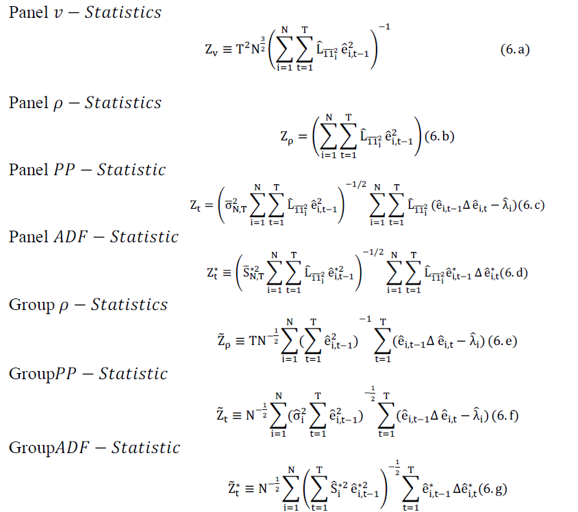 |
| Where, e is the estimated residual from (5) and L is the estimated long-run covariance matrix for Δ e.The other terms are properly defined in Pedroni[43]with the appropriate lag length determined by the Newey–West method. |
ESTIMATING THE LONG RUN COINTEGRATION RELATIONSHIP IN A PANEL CONTEXT |
| After confirmation of the existence of a Co-integration relationship between the series, must be followed by the estimation of the long-term relationship. There are different estimators available to estimate a vector Co-integration panel data, including with and between groups such as OLS estimates, fully modified OLS (FMOLS) estimators and estimators dynamic OLS (DOLS).In the Co-integrated panels, using the technique of ordinary least squares (OLS) to estimate the long-term equation leads to biased parameter estimates unless the regressors are strictlyexogenous, so that, the OLS estimators cannot generally be used for valid inference. |
THE FULLY MODIFIED OLS (FMOLS) AND DYNAMIC OLS (DOLS) ESTIMATORS |
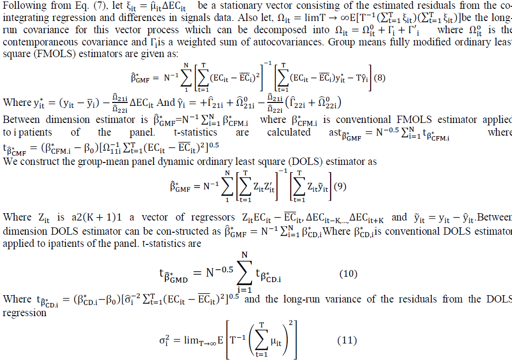
| Pedroni [45] proposes fully modified ordinary least squares (FMOLS) while Kao and Chiang [46] and Mark and Sul [47] recommend the dynamic ordinary least squares (DOLS) as alternative methods of panel co-integration. FMOLS is a non-parametric approach, which takes into account the endogeneity, serial correlation and cross-sectional heterogeneity, and will propose both between dimension and within-dimension estimations. Specifically, the betweendimension estimations are more applicable to small sample. |
| In order to obtain an unbiased estimator of the long-run parameters and to achieve the endogeneity correction, DOLS estimator uses parametric adjustment to the errors by including the past and the future values of the differenced I (1) regressors. |
| Both FMOLS and DOLS provide consistent estimates of standard errors that can be used for inference. According to Kao and Chiang (2000), FMOLS and DOLS estimators have normal limiting properties. The DOLS and FMOLS estimations are given by the following equation: |
 |
| Where yrepresents ECG, ECrepresents all other signals and y and EC are cointegrated with slopes β, which may or may not be homogeneous across i. |
 |
PANEL GRANGER CAUSALITY |
| Panel Co-integration method tests whether the existence or absences of long-run relationship between cardiorespiratory hemodynamic signals for the 186 patients. It doesn't indicate the direction of causality. When Co-integration exists among the variables, the causal relationship should be modeled within a dynamic error correction model Engle and Granger [4]. The main purpose of our study is to establish the causal linkages between cardiorespiratory hemodynamic signals, the Granger causality tests will be based on the following regressions: |
 |
| X can take ECG Three Leads, in other words X= {ECG Lead 1, ECG Lead 2 or ECG Lead 3} are as previously defined, ECT is the error-correction term,p denotes the lag length and (1 − L)is the first difference operator and ECT stands for the lagged error correction term derived from the long-run cointegration relationship. An error correction model enables one to distinguish between the long-run and short run Granger causality. The short term dynamics are captured by the individual coefficients of the lagged terms. Statistical significance of the coefficients of each explanatory variable are used to test for the short run Granger causality while the significance of the coefficients of ECT gives informationabout long-run causality. It is also desirable to test whether the two source of causation are jointly significant. |
EMPIRICAL RESULT |
| Before beginning our results, we must clarify some details and signs: |
| Corresponds to the causal direction between three ECG leads to (ART, CVP, PAP, RESP, and CO2). |
| Corresponds to the causal direction between (ART, CVP, PAP, RESP, and CO2) to three ECG leads. |
| *: Indicates statistical significance at 1%. |
| A Value above the sign , is the value of |
| F-statistic, which is considered a measure of the correlation between the variables studied. |
| A value above the sign , which is in brackets, corresponds to the value of the probability of causation. |
| (x E x) : (x exponential x). |
| MGH Number: corresponds to a given patient. |
| [x: long-term coefficient. |
A. Panel unit root tests |
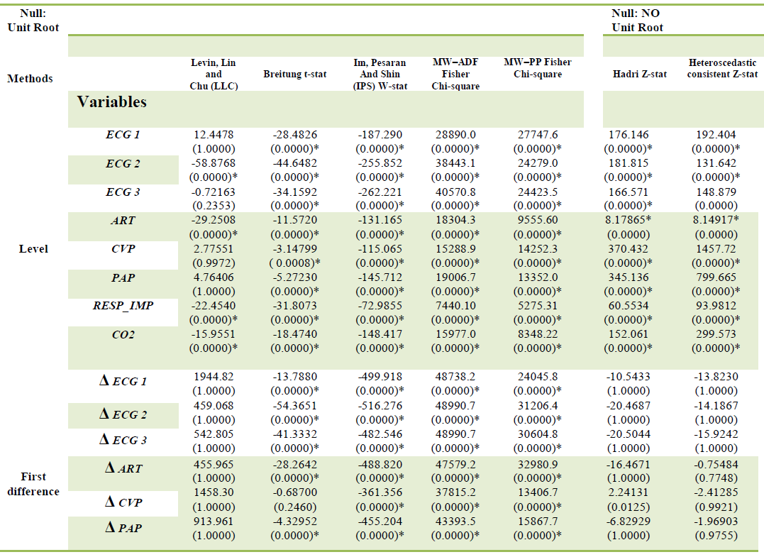
| To investigate the stationarity of the used series, we used the unit root tests on panel data (Levin Lin and Chu[37], IM Pesaran and Shin[38],Breitung, Maddala and Wu[39]). The results of these tests are presented in the TAB I |
 |
 |
| The table summarizes the results of tests (LLC), (IPS), (BRT), (MW) and Hadri test applied to the variables of the model. (LLC) Tests and especially the Hadri test show that the series are non-stationary in level; other tests indicate that all series are stationary in level. This contradiction in the results leads us to the test in first differences, to ensure the integration of variable order. Passing the first differences, we find that all series are stationary, even for Hadri test. We conclude that they are integrated of order one I {(1)}. |
| Set apart the (LLC) test, which indicates that the series are non-stationary in first differences; this can be partly explained by the low statistical power of this test providing the other unit root tests used as the Hadri test. We can nevertheless emphasize the efficiency and power of unit root tests in panel, as in the first series are stationary differentiation whatsoeverfor the model with trend and constant, constant or neither constant nor trend. This proves that the panel tests are more powerful compared to unit root tests in time series. |
B. Panel Co-integration results |
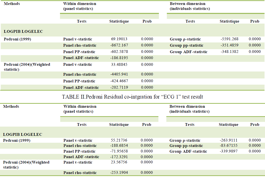
| We have seen that all variables are integrated order oneI, Based on these test results panel unit root, we proceed to Cointegration test panel and that by relying on Pedronitests[43, 44, 45].TAB II, III, IV shows the outcomes of Pedroni's[43]Co-integration tests between the cardiorespiratory hemodynamic signals. We use four within group tests and three between-group tests to check whether the panel data are Co-integrated.The columns labeled within-dimension contain the computed value of the statistics based on estimators that pool the autoregressive coefficient across different patients for the unit root tests on the estimated residuals. The columns labeled between-dimension report the computed value of the statistics based on estimators that average individually calculated coefficients for each patients,the results are as follows: |
 |
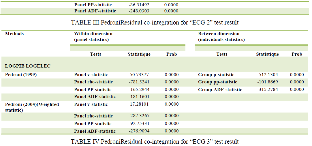 |
| The tables summarize the results of seven PedroniCo-integration statistical. The results show that there is a long-term relationship between the variables in the models studied; this relationship is characterized by a statistically significant and exceptional strength, as all statistical probabilities are equal to 0. So we can say with certainty that there can be noambiguity about the existence of a long-term relationship. Co-integration of variables depends on the value of the probability associated with each statistics. And the seven tables of the three statistical seven probability values are below 1%. These are all integrand intra-individual tests; all this proves that there is a relationship of co-integration between the variables in the model.Estimators give different results. It is important to note that the DOLS method has the disadvantage of reducing theSince our sample size is important, especially in the temporal dimension, the DOLS estimation can give acceptablenumber ofdegrees of freedom by including leads and lags in the studied variables, which leads to less reliable estimates. |
C. The FMOLS and DOLS estimations |
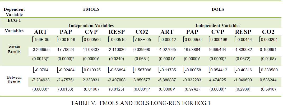
| In this step, we estimate the long-term relationships using FMOLS methods and DOLS estimators proposed by Pedroni [45], Kao and Chiang [46]and Mark and Sul [47]. These results FMOLS and DOLS test results are presented in the following table: |
 |
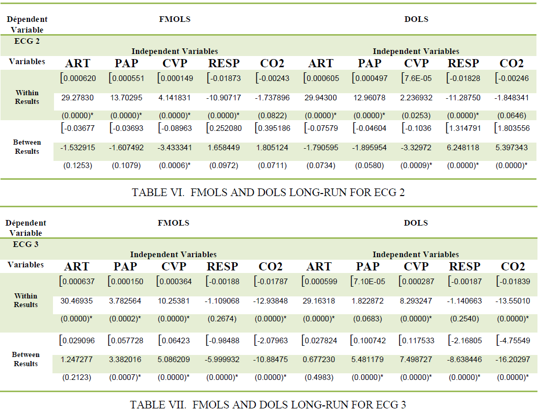 |
| As mentioned above, we used two techniques for obtaining estimates of parameters of the long-term relationship between the three leads ECG and hemodynamic respiratory signals, the TAB V, VI and VII presents the results FMOLS and DOLS. The coefficients of hemodynamic respiratory signals and the three leads ECG1, ECG2 and ECG3, are generally statistically significant at 1% in both within and between. Being the coefficients can be interpreted as elasticity. Overall, the results of this study show that there isastrong long-term relationship between the three leads ECG and hemodynamic respiratory signals. The results for ECG1 ECG2 and ECG3 suggest that an increase of 1% of PAP increases ECG’s, respectively, 0.001016 % 0.000551 % 0.000150 % in the Within dimension based on the method FMOLS, these results highlight the involvement of hemodynamic signals to three ECG leads. These resultssuggest that a 1% increase in CVP increases ECG1 and ECG3, respectively, 0.054412 % 0.117533 % in the between dimension based on the DOLS method. It should be noted that the coefficients as (ART, RESP, and CO2) are negative, in this case must take its results with the greatest caution. |
D. Panel Granger causality results |
| Having established that the three leadsECG is Co-integrated in the long-term with hemodynamic respiratory signals, this step is done to objectively examine the causal relationship between these variables, the following table summarize all the results of causality, the optimal structure of delays was established using the Akaike and Schwarz information criteria. |
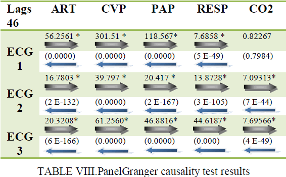 |
| The table shows that there is a cause and effect way, except in the case ECG1 with CO2, or where there's no causality, summary Granger causality runs from three ECG leads to hemodynamic respiratory signals for different individuals and vice versa. In other words, the assumption of feedback (bidirectional relationship between three lead ECG and hemodynamic signals in which the causality works in both directions) is confirmed for these individuals. Therefore, any impact from the hemodynamic respiratory signals will affect the three ECG leads and vice versa. |
DISCUSSIONS AND CONCLUSIONS |
| In order to check the long-term convergence between our studied signals, we applied the Co-integration method. The results show that there is actually a convergence of these signals. In this article, we focus on the technical and non-medical aspects in the fact that we belong to the telemedicine fields, however we will give some scientific explanations to clarify this convergence. First, pulmonary hypertension in the long-term, it causes right ventricular failure. Second, blood hypertension induced left ventricular hypertrophy that will cause at long-term a heart failure. Finally, a sufficient supply of oxygen to the heart, weak and overloaded will cause at long-term coronary heart disease. |
| Our hypotheses are based and validated by the Granger causality and Co-integration panel in long-run, the mathematically search result obtained by this method could confirm the cardiorespiratory hemodynamic anatomy, the knowledge and the quantitative understanding of these interactions are critical in monitoring people at risk situations (awakening from anesthesia, age-related pathologies, followed pregnant women, …), so for our future telemedicine applications, is a real progress towards the perfect analysis of signals received in real time and in long-term. Based on these results, we will draw in advance and with the inclusion of all the interdependencies with these specific degrees protocols enable an excellent Intervention. |
CONFLICT OF INTEREST |
| An earlier version of this paper was presented at the WCCAIS 2014 IEEE Conference, Hammamet, Tunisia, January 17-19, 2014. Our paperentitled“Causal relationships between cardiorespiratory hemodynamics signals: Test analysis using panel Co-integration” was selected by the Conference as one of its top papers; we will present now our extended version. |
References |
|