ISSN ONLINE(2320-9801) PRINT (2320-9798)
ISSN ONLINE(2320-9801) PRINT (2320-9798)
Soma Datta 1, Dr. Samir Kumar Bandyopadhyay2
|
| Related article at Pubmed, Scholar Google |
Visit for more related articles at International Journal of Innovative Research in Computer and Communication Engineering
The goal of this work is to development an Image Processing technique to segment patterns from the MRI brain images. The main focus is to automate the segmentation of MRI images that will be fed to the diagnoses unit for automatic classification and report generation. This work also aims to enhancing the images for visual inspection by reducing noise and histogram equalization..
Keywords |
| Laplacian Filter, HIS color format, Euclidean space, Erosion, MRI Images, BMP image format |
INTRODUCTION |
| MRI imaging plays a major role to decide treatment strategy especially for brain injuries. Brain injuries leads several neurological disorder, which can be avoided by early diagnosis and treatments. Traumatic brain injury (TBI) is a serious public health problem in the world. Each year, traumatic brain injuries contribute to a substantial number of deaths and cases of permanent disability. Every year, at least 1.7 million TBIs occur either as an isolated injury or along with other injuries in United States [1][2]. Moreover it is very difficult to arrange sufficient radiologist in emergency situation, like war [3], earthquake etc, to provide treatment for the injured people. It will be very helpful if an alternative process for detection of the nature of the brain injuries by which hazardous clinical examinations more or less can be avoided. The rest of the paper is arranged as follows: section II contains the detail design including hardware design; section III focuses the results and performance of the system and section IV is used to discuss the future scope and overall performance of the system. |
DETAIL DESIGN |
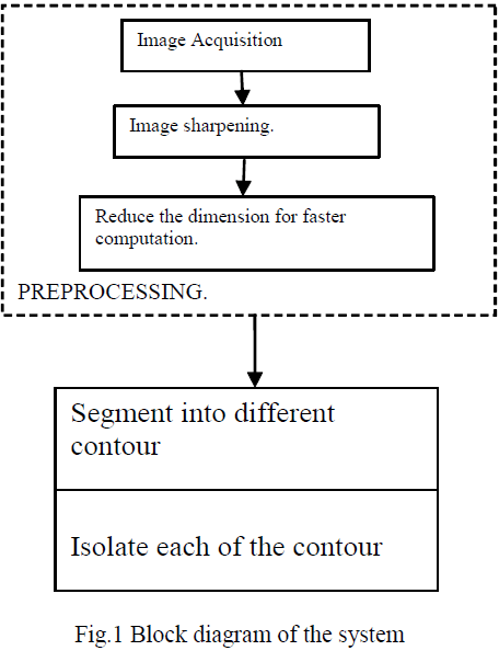
| The entire work is an application of Image Processing and it is divided into several parts like image enhancement , dimension reduction segmentation etc. Fig 1 shows the block diagram of the system. In the pre-processing part the region of interest is segmented from the sharpened image. |
A. Image Acquisition |
| Image Acquisition is the first step of this work. Digitized images of the MRI [10] brain are fed into the system. The system accepts variety of image formats like BMP (bit map format), JPEG (Joint Photographic Experts Group), PNG (Portable Network Graphics) [4] etc. this is because different vendorâÃâ¬ÃŸs MRI machine supports different formats. |
B. Image Enhancement |
| Sometimes the images obtained from the MRI machine are not of good quality. Laplacian Filter [7] is used to sharpen the edges of the objects in the image. |
| The Laplacian value for a pixel is denoted by f(x, y) 2 and it is defined as. |
 |
| This expression is implemented at all points (x,y) of the image through convolution. The Laplacian filter is applied separately on Red, Green and Blue components of the colour image obtained from the device. |
C. Reduce the Dimension of the Image Matrix |
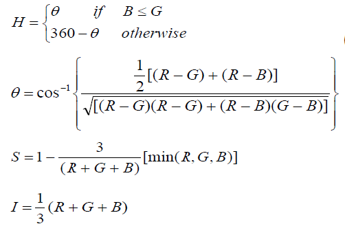
| Most of the input images are in RGB format that means they are in 3 dimensional matrixes. So to save computation time the images converted in to gray images using HIS color format and accept I for further processing and discard other components. In HIS color format H stands for Hue (Pure colour), S for saturation, i.e. the degree by which the pure colour is diluted by white light and I for intensity (Gray level) The RGB to HSI colour space [5][6] conversion process is performed using the equations. |
 |
 |
 |
 |
| D. Segmentation |
| The first step in segmentation [8] is to isolate brain and non brain region and fill the non brain region with a threshold value so that in next stage of segmentation this non brain region will have no influence. The gray scale intensity of MRI images varies case to case; so it is not possible to set a unique threshold value to segment brain and non-brain region. To overcome this problem a relative threshold value [9] selection algorithm is proposed. |
| Algorithm 1: To Calculate relative threshold value. |
| This algorithm is used to calculate the threshold value which will be used to convert the gray image into binary image. |
| Step 1: Select an initial estimate for T (T=threshold value). The initial value for T is the average gray level of the image |
| Step 2: Segment the images using T. This will produce two groups of pixels: consisting of all the pixels with gray level values > T called as G1 and consisting of pixels with values <= T called as G2. |
| Step 3: Compute the average gray level values μ1 and μ2 for the pixels in regions G1 and G2. |
| Step 4: Compute a new threshold value: |
| T = 0.5 * (μ1+ μ2). |
| Step 5: Repeat steps 2 through 4 until the difference in T in successive iterations is smaller than a predefined parameter T0 |
| Step 6: Stop. |
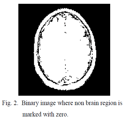
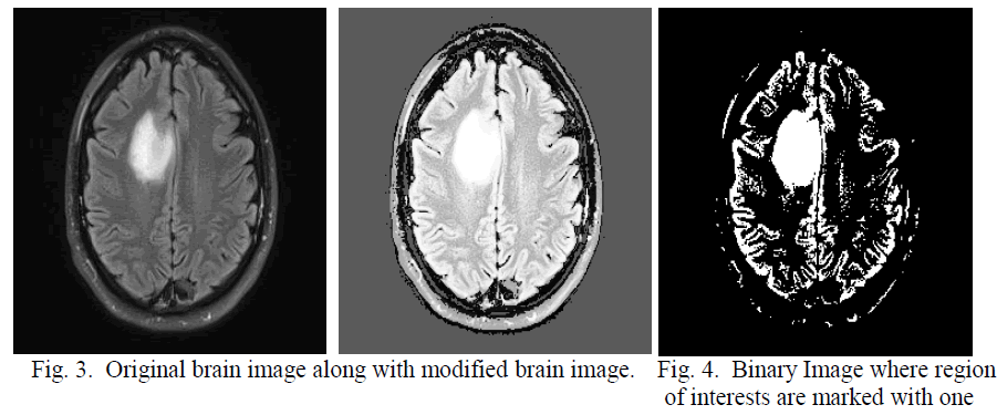
| After obtaining the threshold value the brain image is converted in to binary image in which non brain region is marked with zero, shown in figure 2. The main gray image is modified by feeling the threshold value in the non brain regions so that in the next threshold calculation this non brain region will have less impact shown in figure 3. Using this threshold technique convert the modified image into binary this is shown in the figure 4 In the binary image some unnecessary contours exist; which are actually noise. This noise are eliminated by erosion [11]; discussed in eq 6-7. |
| Let E be a Euclidean space [12] or an integer grid, and A a binary image in E. The erosion of the binary image A by the structuring element B is defined by: |
 |
| When the structuring element B has a center (e.g., a disk or a square), and this center is located on the origin of E, then the erosion of A by B can be understood as the locus of points reached by the center of B when B moves inside A. For example, the erosion of a square of side 10, centered at the origin, by a disc of radius 2, also centered at the origin, is a square of side 6 centered at the origin. Figure 5 shows the eroded image. |
| After that individual contours in the binary image are segmented by label matrix technique. This is done by the following algorithm. |
| Algorithm 2: To find out separate contours. |
| This algorithm is used to segment the valid contours of the binary image shown in fig 5. |
| Step1: Apply label matrix technique in the binary image, and store the output matrix in LB variable. LB will have the same dimension as the binary image. The value „1âÃâ¬ÃŸ in each contour in the binary image will be replaced by an integer number in the LB. |
| Step 2: count = maximum integer value stored in LB; So “count” will contain the number of contours in the input image. |
| Step 3: index = 1 |
| `Step 4: val = maximum gray level value of the pixels in the modified brain image. |
| Step 5 : Find the coordinates of the pixels of the LB where value of the pixel == index; |
| Step 6: local_Value = maximum gray level value of the pixels in the modified brain image whose coordinates are selected in step 5. |
| Step 7: if local_Value > 0.85* val the contour is valid and segment the contour for processing. |
| Else |
| Not a valid contour |
| Step 8 : index = index + 1; |
| Step 9: Repeat step 5 to step 8 until index > count |
| Step 10 : Stop |
| After applying algorithm 2 the valid contours are thickened to compensate the area of the region of interest which are erode earlier; this is shown in figure 6. |
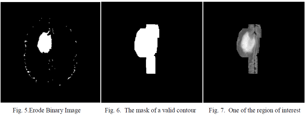 |
| Multiply the mask with the modified gray image [14]. This is shown in figure 7. The sub images will be fed to the decision making units for diagnosis. |
SIMULATION AND RESULTS |
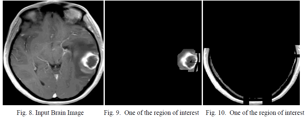
| For simulation MatLab [13] is used. For the particular MRI image shown in fig 3; the result is correct. For another MRI image the segmentation are correct. Fig 8 shows the input image. Fig 9 and fig 10 shows the region of interests. In testing the system have been tested for 150 times and in which 144 give satisfactory results. So the accuracy is 96% |
 |
CONCLUSION |
| This system is efficient and easy to use. It is easy to install. It can reduce the probability wrong diagnosis, and overhead of the radiologist. However this approach provides 96% accuracy, as a next phase of work we are trying to automate the diagnosis part. |
ACKNOWLEDGMENT |
| Authors are thankful to Mr. Pramit Ghosh and physician Dr. Saumendu Datta for providing clinical data and the Department of Computer Science & Engineering, West Bengal University of Technology, for providing infrastructural facilities during progress of the work. |
References |
|