Department of Mathematics and Statistics, University of agriculture Faisalabad, Pakistan
Received date: 19/04/2017 Accepted date: 06/06/2017 Published date: 07/06/2017
Visit for more related articles at Research & Reviews: Journal of Statistics and Mathematical Sciences
The purpose of this paper is to introduce a size biased Lindley distribution. Size biased distribution is a special case of weighted distributions. Weighted distributions have practical significance in situations where units in population do not follow the exact distribution from which they are supposed to belong. That means some types of biased occur in a density function and most commonly the units are size biased in certain circumstances, which means probability is proportional to the size of the random variable. Lindley distribution has its applications in reliability and lifetime models and in certain situations probability is proportional to size of the variate that’s why the proposed version which is size biased will be modeled such situations more reasonably and more precisely. Major properties of the density function are also discussed in this paper such as moments, measure of skewness and kurtosis, moment generating function, characteristics function, and coefficient of variation, survival function and hazard function which are derived for understanding the structure of the proposed distribution more briefly
Lindley distribution, Weighted distribution, Size biased, Survival function, Hazard function
Weighted Distributions
Weighted distributions are required when the recorded observation from an event cannot randomly sample from actual distribution. This happens when the original observation damaged as well as an event occur in non-observability manner. Due to these inappropriate situations resulting values are reduced, and units or events does not does not have same chances of occurrences as if they follow the exact distribution.
Let the original observation x has pdf f(x) then in case of any biased in sampling appropriate weighted function, say w(x) which is a function of random variable will be introduced to model the situation,
Then new density function (x) will be given by eq. (1), where fw represent a weighted distribution where w is considered as weighted function:
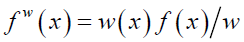 (1)
(1)
Where, w is considered as normalizing factor which is utilized to create total probability or area under the curve, equal to 1. If w(x) is constant term then fw(x)=f(x).
The Lindley distribution Shanker et al. introduced with two parameters by taking in to account the survival and waiting time data. In Lindley, exponential distribution Bhatti and Malik [1] studied its mathematical properties and check its flexibility by using real data set. Due to one parameter of Lindley distribution Zakerzadeh and Dolati stated that it does not support for the better analysis of life time data they provide family of distribution with three parameters which is more flexible for modeling of life time data. The geometric Lindley was extended by Mervoci and Elbatal into a new model called transmuted geometric Lindley. Lindley distribution and exponential distribution was compared by Ghitany et al. in which it is concluded that model provide effective conclusion and they also check the flexibility of their properties. Poisson Lindley distribution was enlarged by Borah and Deka Nath [2-4] with further study called inflated poisson Lindley distribution. Ghitany et al. comes up with a comparison of two models and showed that Lindley distribution provide effective model than exponential distribution. Whereas Ghitany et al. [5-8] examined the poisson Lindley distribution to model count data, as well as Ghitany et al. aims their study for data does not include zero counts, since Zakerzadeh and Dolati described generalized form of Lindley distribution with three parameters. Therefore, Ghitany et al. worked on modeling of survival data and introduced a Lindley distribution with two parameters called weighted Lindley distribution although Lord and Geedipally [9] proposed a new distribution called negative binomial Lindley, contains two parameter for crash count data. Mazcheli and Achcar worked on competing risk data. Bakouch et al. proposed extended form of Lindley distribution to model the life time data to check its reliability, failure rate function. Whereas Elbatal et al. [4] proposed that Lindley distribution is a mixture of both gamma and exponential distribution. Shanker et al. compared one parameter Lindley distribution with two parameter Lindley distribution while Wang introduced a life time distribution with three parameters. although Bhati and Malik worked at Lindley random variable and bring in to being a new family of distribution distribution for remission times uncensored data of 128 cancer bladder patients Mervoci and Sharma [11-15] extended the Lindley distribution called beta Lindley distribution. Whereas Singh et al. [16] give truncated Lindley distribution.
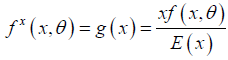
The idea of moments distributions which are most commonly used weighted distributions in literature is used to find out the size biased pdf of the Lindley distribution. where for size biased [12-18] distribution x is taken as weighted function for f(x) and normalizing factor is E(x) to make total area is to be 1.
Mathematically,
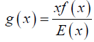
Where x is a weighted function f(x) is the actual pdf and E(x) is the mean of original density function and g(x) represents the size biased density function.
Some structural properties discussed by using simple algebraic methods whereas some results of original and size biased density function are compared based on random samples for each density function. For data simulation and calculation of results based on these samples r programming language is used. Both functions are compared based on these results of simulation, for different values of parameter θ .
One Parameter Lindley Distribution
A one parameter Lindley distribution with parameter θ is defined by its probability density function is given as (Figure 1):

Figure 1. Graphical behavior of Lindley distribution for some values of parameter.
 (2)
(2)
Plot of Probability Function of Lindley Distribution
Raw Moments
The rth moments about origin of one parameter Lindley distribution is given by eq. (3)
 (3)
(3)
Taking r=1, 2, 3 and 4 in this equation the first four moments about origin is obtained as:
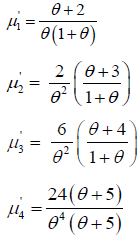
Moments about Mean of One Parameter Lindley Distribution
Then central moments are obtained as (Table 1),
| Lindley distribution |
Std. Dev | ||||
|---|---|---|---|---|---|
| = 0.1 | 19.09091 | 199.1736 | 3998.497 | 239006.2 | 14.11289 |
| = 0.5 | 3.333333 | 7.555556 | 31.40741 | 362.0741 | 2.748737 |
| = 0.9 | 1.695906 | 2.192127 | 5.195381 | 32.24576 | 1.480583 |
| = 1.3 | 1.103679 | 0.994396 | 1.656285 | 6.953597 | 0.9971941 |
| = 1.7 | 0.8061002 | 0.5548673 | 0.712556 | 2.247497 | 0.7448942 |
| = 2.1 | 0.6298003 | 0.3494565 | 0.3647844 | 0.9184176 | 0.5911485 |
| = 2.5 | 0.5142857 | 0.2383673 | 0.2093528 | 0.4376736 | 0.4882287 |
| = 2.9 | 0.4332449 | 0.1720659 | 0.1302924 | 0.2325485 | 0.4148083 |
| = 3.3 | 0.3735025 | 0.1295714 | 0.08615088 | 0.1340034 | 0.3599603 |
Table 1. Central moments and standard deviation for different values of parameter θ .
Cumulative distribution function of Lindley distribution
Cdf of the Lindley distribution is given by eq. (4): (Figure 2).

Figure 2. Graphical behaviors of cumulative density function of the Lindley distribution.
This gives,
 (4)
(4)
Plot of Cumulative Distribution Function of Lindley Distribution
Moment generating function of Lindley Distribution:
Characteristic generating function of One Parameter Lindley Distribution is given by:
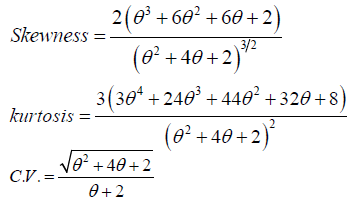
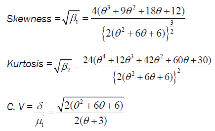
Skewness, Kurtosis and Coefficient of Variation of Lindley Distribution is given in Table 2 as:
| Skewness | Kurtosis | C.V | |
|---|---|---|---|
| 0.1 | 1.42249 | 6.024845 | 0.7392464 |
| 0.5 | 1.512281 | 6.342561 | 0.8246211 |
| 0.9 | 1.600732 | 6.710286 | 0.8730337 |
| 1.3 | 1.670306 | 7.032192 | 0.9035183 |
| 1.7 | 1.723992 | 7.299966 | 0.9240714 |
| 2.1 | 1.765821 | 7.520627 | 0.9386284 |
| 2.5 | 1.798906 | 7.702946 | 0.9493337 |
| 2.9 | 1.825478 | 7.854595 | 0.9574452 |
| 3.3 | 1.847123 | 7.981736 | 0.9637429 |
Table 2. Skewness, kurtosis and coefficient of variation for some values of parameter θ.
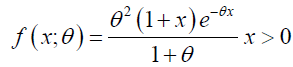
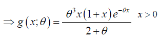
Size Biased Lindley Distribution
The probability density function of size biased Lindley distribution is given as (Figure 3):

Figure 3. Graphical behavior size biased density function for some values of parameter.
 (5)
(5)
Plot of probability function of size Biased Lindley Distribution
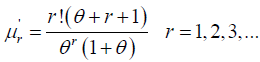
Raw Moments of Size Biased Lindley Distribution
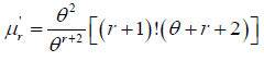 (6)
(6)
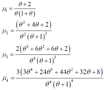
Taking r=1,2,3 and 4 in this equation the first four moments about origin is obtained as
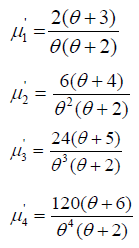
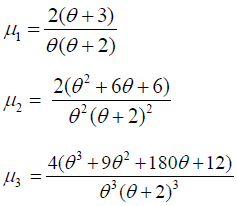
Moments about Mean of Size Biased Lindley Distribution
Central moments of size biased Lindley distribution is obtained in Table 3 as:
| SBLD | µ1 | µ2 | µ3 | µ4 | Std. Dev |
|---|---|---|---|---|---|
| θ=0.1 | 29.52381 | 299.7732 | 5999.784 | 449591.7 | 17.31396 |
| θ=0.5 | 5.6 | 11.84 | 47.872 | 708.4032 | 3.44093 |
| θ=0.9 | 2.988506 | 3.584798 | 8.148448 | 65.90233 | 1.297429 |
| θ=1.3 | 2.004662 | 1.683321 | 2.675344 | 14.75241 | 1.297429 |
| θ=1.7 | 1.494436 | 0.9650163 | 1.181765 | 4.916901 | 0.9823524 |
| θ=2.1 | 1.184669 | 0.6207837 | 0.6188595 | 1.025826 | 0.7878983 |
| θ=2.5 | 0.977778 | 0.4306173 | 0.3620521 | 1.002462 | 0.6562144 |
| θ=2.9 | 0.8304011 | 0.3150689 | 0.2290128 | 0.5418929 | 0.56131 |
| θ=3.3 | 0.7204117 | 0.2398822 | 0.1535249 | 0.3168071 | 0.4897777 |
Table 3. Central moments and standard deviation for different values of parameter θ.
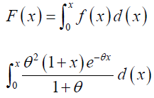
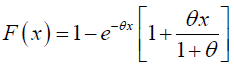
Cumulative Distribution Function of Size biased Lindley Distribution
Cdf of size biased Lindley distribution is given by (Figure 4),

Figure 4. Graphical behavior of cumulative density function of size biased Lindley distribution for some values of parameter.
This gives
 (7)
(7)
Plot of cumulative distribution function of Size biased Lindley
Moment generating function of size biased Lindley distribution:
Characteristics function of size biased Lindley distribution:
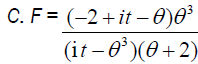
Skewness, Kurtosis and Coefficient of variation of size biased Lindley distribution (Table 4):
| θ | Skewness Size biased | Kurtosis of size biased | Cv Size biased |
|---|---|---|---|
| 0.1 | 1.155969 | 5.003023 | 0.5864406 |
| 0.5 | 1.175044 | 5.053324 | 0.6144518 |
| 0.9 | 1.200544 | 5.128277 | 0.6335461 |
| 1.3 | 1.224981 | 5.206302 | 0.6472056 |
| 1.7 | 1.246606 | 5.279858 | 0.6573401 |
| 2.1 | 1.265265 | 5.34658 | 0.6650788 |
| 2.5 | 1.28125 | 5.406111 | 0.6711283 |
| 2.9 | 1.294946 | 5.458867 | 0.6759504 |
| 3.3 | 1.306718 | 5.505525 | 0.6798582 |
Table 4. Skewness, kurtosis and coefficient of variation, for some values of parameter θ.
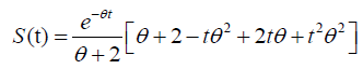
Survival function of size biased Lindley:
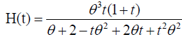
Hazard function of size biased Lindley:
Tables 5 and 6 shows some results of original and size biased Lindley distribution respectively which are based on random samples that are generated for different values of the parameterθ . Each sample is based on 10,000 observations.
| Lindley distribution | Mean | Variance | Standard deviation | Median | Skewness | Kurtosis |
|---|---|---|---|---|---|---|
| θ =0.1 | 17.280 | 128.6998 | 11.34459 | 14.960 | 0.7519824 | 2.899294 |
| θ =0.5 | 3.221 | 7.572646 | 2.751844 | 2.485 | 2.485 | 6.332139 |
| θ =0.9 | 1.610 | 2.119268 | 1.455771 | 1.245 | 1.671199 | 7.427447 |
| θ=1 | 1.403 | 1.582653 | 1.258035 | 1.042 | 1.62406 | 6.789065 |
| θ=1.3 | 1.054 | 0.979174 | 0.9895322 | 0.765 | 1.776654 | 7.588966 |
| θ=1.7 | 0.7706 | 0.5534715 | 0.7439567 | 0.5500 | 1.761394 | 4.358188 |
| θ=2.1 | 0.5875 | 0.3416315 | 0.5844925 | 0.4200 | 1.8265 | 7.129288 |
| θ=2.5 | 0.4656 | 0.2213501 | 0.4704785 | 0.3050 | 2.072667 | 9.192622 |
| θ=2.9 | 0.4014 | 0.1666295 | 0.4082028 | 0.2650 | 2.119914 | 9.657423 |
| θ=3.3 | 0.3386 | 0.1222347 | 0.3496208 | 0.2150 | 2.038068 | 8.910684 |
Table 5. Results based on random samples from Lindley distribution.
| Size biased Lindley distribution | Mean | Variance | Standard deviation | Median | Skewness | Kurtosis |
|---|---|---|---|---|---|---|
| θ =0.1 | 24.570 | 132.92 | 11.5291 | 23.280 | 0.2377253 | 2.158117 |
| θ =0.5 | 5.615 | 12.35464 | 3.514917 | 4.925 | 1.158568 | 5.12711 |
| θ =0.9 | 2.950 | 3.502266 | 1.871434 | 2.550 | 1.278998 | 5.439581 |
| θ=1 | 2.647 | 2.879649 | 1.696953 | 2.310 | 1.265753 | 5.273339 |
| θ=1.3 | 1.974 | 1.617517 | 1.271816 | 1.750 | 1.220679 | 5.268042 |
| θ=1.7 | 1.482 | 0.9617643 | 0.9806958 | 1.330 | 1.052395 | 4.459788 |
| θ=2.1 | 1.160 | 0.6304327 | 0.7939979 | 1.000 | 1.178295 | 5.009183 |
| θ=2.5 | 0.9508 | 0.4314958 | 0.6568834 | 0.7950 | 1.346804 | 6.400068 |
| θ=2.9 | 0.7987 | 0.3249239 | 0.570021 | 0.6800 | 1.240408 | 4.868574 |
| θ=3.3 | 0.6867 | 0.239743 | 0.4896356 | 0.5700 | 1.435663 | 6.086738 |
Table 6. Results based on random samples from size biased Lindley distribution.
Results
By comparing the results in above tables, it is noted that mean, median, and standard deviation all these measures are greater in magnitude for size biased distribution as compared to actual distribution for respective values of parameters. Whereas size biased Lindley distribution is less skewed and less peaked when compare with the original one. Graphical behavior in pdf plots Figures 1 and 3 are also reflecting the same results.