Joseph Justin Rebello*, Shafna Noushad
Department of Statistics, Mahatma Gandhi University, Kerala, India
Received: 16-Jan-2023, Manuscript No. JSMS-23-87204; Editor assigned: 18-Jan-2023, Pre QC No. JSMS-23-87204 (PQ); Reviewed: 01-Feb-2023, QC No. JSMS-23-87204; Revised: 18-Apr-2023, Manuscript No. JSMS-23-87204 (R); Published: 01-Jun-2023, DOI: 10.4172/JSMS.9.2.012
Citation: Rebello JJ, et al. Some Studies on Multivariate Anova and Profile Analysis. RRJ Stats Math Sci. 2023;09:012.
Copyright: © 2023 Rebello JJ, et al. This is an open-access article distributed under the terms of the Creative Commons Attribution License, which permits unrestricted use, distribution and reproduction in any medium, provided the original author and source are credited.
Visit for more related articles at Research & Reviews: Journal of Statistics and Mathematical Sciences
Multivariate Analysis of variance and profile analysis are often used for comparison testing in a multivariate perspective. In this paper, we used a treatment data of a psychological study. The forty patients were randomly assigned to one of four therapies with exactly ten patients per therapy. Three standard instruments were used to assess outcome. These instruments are the Symptom Index for Kleptomania Evaluation (SICE), the Social Functioning for Kleptomania Disorder Inventory (SFCDI), and the Occupational Adjustment Scale (OAS). The three measures were given at two time points, pre and post. Here we check the significant difference of these three measures under the two time points using two different methods repeated measure MANOVA and Profile Analysis. We also check whether the therapies are effective with respect to the given three instruments using repeated measure MANOVA and
profile analysis.
MANOVA; Profile analysis; Hypothesis testing; Likelihood ratio test; Data analysis
This paper we study these two multivariate techniques on the secondary data using a statistical software SPSS [1].
Some researchers have also done some useful work in this area. Cole and Grizzle have provided the use of MANOVA (Multivariate Analysis of Variance) for the analysis of repeated measurement experiments as the successive observations of the same variable are supposed to be correlated.
Khatri presented a note on a MANOVA model applicable to the problems in growth curves for repeated measures data. Wang, et al., fitted a mixed model with repeated measurements using SAS to determine the optimum test duration and the effect of missing data on accuracy of measuring feed efficiency and its four related traits ADG, DMI, feed conversion ratio, and residual feed intake in beef cattle by repeated measurements.
Mendes, et al., used the methods of profile analysis and growth curve analysis to investigate the effect of different feed restrictions applied in 134 journal of reliability and statistical studies, early period on changes of body mass index of ross 308 broiler chickens. Profile analysis was used to compare differences among the groups and the Gompertz growth function was regressed from these data to estimate the growth parameters. Tiwari and Shukla have used the approach of linear mixed model for the analysis of longitudinal data using SAS software [2].
MANOVA
MANOVA is the multivariate analogue of ANOVA. The purpose of MANOVA is to the test equality of mean vectors. That is; to test whether the vectors of means for two or more groups are sampled from the same sampling distribution [3].
Assumptions of MANOVA:
• Multivariate normality: The dependent variable should be normally distributed within groups.
• Linearity: MANOVA assumes that there are linear relationships among all pairs of dependent variables, allpairs of covariates, and all dependent variable covariate pairs in each cell.
• Homogeneity of the covariance matrix: Homogeneity of variances assumes that the dependent variablesexhibit equal levels of variance across the range of predictor variables.
• Independence of observations: Subjects scores on the dependent measures should not be influenced by orrelated to scores of other subjects in the condition or level.
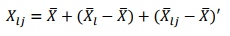
Xlj=μ+τ=elj, j=1,2,…, Nl and l=1,2,…, g
Where elj are independent Np(0,Σ) variables. Here the parameter μ is over all mean and τl represents the lth treatment effect. A vector of observations may be decomposed as suggested by the model (Table 1). Thus,
Let the within sum of squares and cross product matrix be expressed as
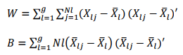
Then the MANOVA table for testing H0: μ1=μ2=.....=μg is given by Table 1.
| Source of variation | Matrix of sum of squares and cross products | Degrees of freedom |
|---|---|---|
| Treatment | 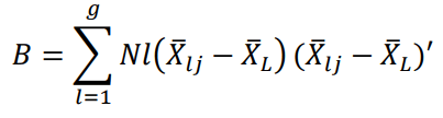 |
g-1 |
| Residual (Error) | 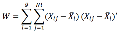 |
 |
| Total | B+W |  |
Table 1. MANOVA table for comparing population mean vectors.
Hypotheses testing in MANOVA
One test of the null hypothesis is carried out using a statistic called Wilk's Λ (a likelihood ratio test);
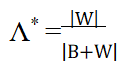
We reject the null hypothesis when Λ* is small.
Profile analysis
In profile analysis data is plotted with time points along the X-axis with scores or responses along Y-axis let μ=(μ1, μ2, …, μp)′ be the mean score vector for a population. The graph obtained by plotting (1, μ1), (2, μ2) …. (p, μp) and joining them by line segment is called the profile of the population (Figure 1) [4].

Figure 1: Profile plot.
Assume that two populations follow multivariate Normal distribution (Figures 2-4). In profile Analysis we examine whether the average effects of various tests are same for both the populations. i.e., with the same multivariate normal populations Np(μ(i), Σ), i=1,2…Three general hypotheses in profile analysis:
H01: The profiles for these groups are parallel.
H02: Same average response level.
H03: Effects of P tests is same in both the populations (Figure 2).
Take 2 independent random samples of sizes Ni from two multivariate normal populations.
Np(μ(i), Σ) for i=1,2
Test (parallel)
Test statistic is,
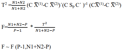
Confidence region is F ≤ Fα (Figure 2).

Figure 2: Comparison of two profiles under the hypothesis of parallelism.
Test (Level)
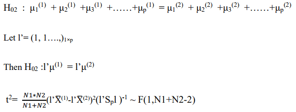
Confidence region is F ≤ Fα (Figures 3 and 4).

Figure 3: Hypothesis H02 of equal group effect without parallelism.

Figure 4: Hypothesis H02 of equal group effect, assuming parallelism.
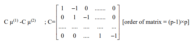
Test (Coincidences)
Need to proceed with test 3 only if H01 and H02 are true (Figure 5).
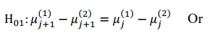
H03: μ1(1)+μ1(2)=μ2(1)+μ2(2)=……..=μp(1)+μp(2)
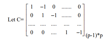
Then H03: C(μ(1)+μ(2))=0
Test statistic is,
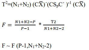
Confidence region is F ≤ Fα

Figure 5: Hypothesis H03 of equal tests (variables) assuming parallelism.
Nature of the data
Patients for this study were forty males between the ages of 21 and 60 who were consecutive admissions to the Waldo Jones Kleptomania clinic and were independently diagnosed by two clinicians as meeting the American psychiatric association’s diagnostic and statistical manual, V edition (provisional), criteria for kleptomania disorder.
The forty patients were randomly assigned to one of four therapies with exactly ten patients per therapy. The first therapy, termed the control therapy here, was the traditional approach to kleptomania taken in the clinic. The remaining three therapies were experimental treatments. Therapy number two, the first of the experimental treatments, was a cognitive therapy in which the patients were to read daily a statement that told them they were really good people. Therapy number three used a behavioural modification approach. The final therapy was based on abreaction principles [5].
Three standard instruments were used to assess outcome. These instruments are the Symptom Index for Kleptomania Evaluation (SICE), the Social Functioning for Kleptomania Disorder Inventory (SFCDI), and the Occupational Adjustment Scale (OAS). The three measures were given at two time points. The first time point, termed the pre-test herein, was when patients entered the clinic and before assignment to one of the four treatments. The second time point, the post-test, occurred exactly two weeks after the start of treatment (Table 2) [6].
| Variable name: | Description |
|---|---|
| Subject | Subject number within group |
| Group | Numeric index of group |
| Therapy | Character index of group |
| SI_pre | Symptom Index for kleptomania evaluation: Pre-test |
| SF_pre | Social functioning for kleptomania disorder inventory: Pre-test |
| OA_pre | Occupational adjustment scale: Pre-test |
| SI_post | Symptom index for kleptomania evaluation: Post-test |
| SF_post | Social functioning for kleptomania disorder inventory: Post-test |
| OA_post | Occupational adjustment scale: Post-test |
Table 2. Shows variable name and their description.
Analysis of data
Repeated measure MANOVA: H0: There is no significant difference over the three instruments due to the therapies at two different time points (Table 3).
| Within subjects effect | Value | F | Hypothesis df | Error df | Sig. | |
|---|---|---|---|---|---|---|
| Time | Pillai's trace | 0.684 | 24.500c | 3 | 34 | 0 |
| Wilks' lambda | 0.316 | 24.500c | 3 | 34 | 0 | |
| Hotelling's trace | 2.162 | 24.500c | 3 | 34 | 0 | |
| Roy's largest root | 2.162 | 24.500c | 3 | 34 | 0 | |
| Time*group | Pillai's trace | 0.631 | 3.198 | 9 | 108 | 0.002 |
| Wilks' lambda | 0.464 | 3.413 | 9 | 82.898 | 0.001 | |
| Hotelling's trace | 0.95 | 3.446 | 9 | 98 | 0.001 | |
| Roy's largest root | 0.638 | 7.659d | 3 | 36 | 0 | |
| Note: c: Exact statistic; d: The statistic is an upper bound on F that yields a lower bound on the significance level. | ||||||
Table 3. Multivariate.
SPSS Produces different tables on analysis of Repeated measure MANOVA. From which the above table shows whether the MANOVA is statistically significant. That is whether the measures are significantly different with respect to the given time points. The "Sig." column presents the significance value (i.e., p-value) of the one-way repeated measures MANOVA.
If p<.05 (i.e., if p is less than .05), the one-way repeated measures MANOVA is statistically significant. Alternatively, if p>.05 (i.e., if p is greater than .05), the one-way repeated measures MANOVA is not statistically significant.
Here the p-value is 0.000 which means our three measures namely, Symptom Index for Kleptomania Evaluation (SICE), the Social Functioning for Kleptomania Disorder Inventory (SFCDI), and the Occupational Adjustment Scale (OAS) differs at the two time points pre and post; that is before different therapies and after the therapies [7].
Profile analysis
The profile plots of Symptom Index for Kleptomania Evaluation (SICE), the Social Functioning for Kleptomania Disorder Inventory (SFCDI), and the Occupational Adjustment Scale (OAS) at two different time points (Before therapies and after therapies) are given below (Figures 6-8).

Figure 6: Profile plots for Symptom Index for Kleptomania Evaluation (SICE).

Figure 7: Profile plots for the Social Functioning for Kleptomania Disorder Inventory (SFCDI).

Figure 8: Profile plots for the Occupational Adjustment Scale (OAS).
Clearly these three graphs show that the null hypothesis
H01: The profiles for these groups are parallel.
H02: Same average response level and
H03: Effects of P tests is same in both the populations are rejected.
That is measures are significantly different with respect to the given time points [8].
SPSS output on testing parallelism and response level in profile analysis
Here the test of parallelism indicates that parallelism is rejected since F(1,36)=2.270,7.541,1.841 is greater than the p value 0.116 respectively for si, sf and oa. The values F(1,36)=38.045, 70.677,26.189 are also greater than p value=0.003987 which indicates the rejection of H02 (Table 4).
| Source | Measure | Time | Type III sum of squares | df | Mean square | F | Sig. |
|---|---|---|---|---|---|---|---|
| Time | si | Linear | 1344.8 | 1 | 1344.8 | 38.045 | 0 |
| sf | Linear | 2928.2 | 1 | 2928.2 | 70.677 | 0 | |
| oa | Linear | 696.2 | 1 | 696.2 | 26.189 | 0 | |
| Time*therapy | si | Linear | 240.7 | 3 | 80.233 | 2.27 | 0.097 |
| sf | Linear | 937.3 | 3 | 312.433 | 7.541 | 0 | |
| oa | Linear | 146.8 | 3 | 48.933 | 1.841 | 0.157 | |
| Error (time) | si | Linear | 1272.5 | 36 | 35.347 | ||
| sf | Linear | 1491.5 | 36 | 41.431 | |||
| oa | Linear | 957 | 36 | 26.583 |
Table 4. Tests of within-subjects effects.
Now we get the output on testing the hypothesis H03: Same average response level as follows in Table 5.
| Transformed variable: Average | ||||||
|---|---|---|---|---|---|---|
| Source | Measure | Type III sum of squares | df | Mean square | F | Sig. |
| Intercept | si | 237402.1 | 1 | 237402.1 | 2044.171 | 0 |
| sf | 253350.1 | 1 | 253350.1 | 1428.554 | 0 | |
| oa | 223661.3 | 1 | 223661.3 | 1179.406 | 0 | |
| Therapy | si | 95.05 | 3 | 31.683 | 0.273 | 0.845 |
| sf | 612.45 | 3 | 204.15 | 1.151 | 0.342 | |
| oa | 121.75 | 3 | 40.583 | 0.214 | 0.886 | |
| Error | si | 4180.9 | 36 | 116.136 | ||
| sf | 6384.5 | 36 | 177.347 | |||
| oa | 6827 | 36 | 189.639 | |||
Table 5. Tests of between subjects effects.
Here the test of coincidence indicates that H03 is rejected since F(3,36)=0.273,1.151,0.214 is greater than the p value 0.116 respectively for si, sf and oa. As the three hypotheses are rejected, we can clearly say that there is significant difference over the three instruments due to the therapies at two different time points [9,10].
The repeated measure MANOVA led to the conclusion that there is significant difference over the three instruments due to the therapies at two time points. That is the therapies are effective with respect to the three instruments Symptom Index for Kleptomania Evaluation (SICE), the Social Functioning for Kleptomania Disorder Inventory (SFCDI), and the Occupational Adjustment Scale (OAS). Since for all the four test statistics (Wilk’s Lambda, Pillai’s trace, Hotelling-Lowley trace and Roy’s largest root statistics) both time effect and time*therapy effect were found to be significant. Profile analysis was done to test the hypothesis parallelism, response level and coincidence. The findings reveals that all the three hypotheses are rejected which indicates that there is significant difference among the two time points with respect to the three instruments. Thus, profile analysis led to the similar results as revealed by the repeated measure MANOVA.
[Crossref]
[Crossref] [Google Scholar] [PubMed]