Spatial Information Based Image Classification
Using Support Vector Machine

P.Jeevitha; Dr. P. Ganesh Kumar

Spatial Information Based Image Classification Using Support Vector Machine

P.Jeevitha, Dr. P. Ganesh Kumar

PG Scholar, Dept of IT, Regional Centre of Anna University, Coimbatore, India.
Assistant Professor, Dept of IT, Regional Centre of Anna University, Coimbatore, India

Related article at Pubmed, Scholar Google

Visit for more related articles at International Journal of Innovative Research in Computer and Communication Engineering

Abstract

Segmentation and classification of images are major task of remote sensing. Active learning approach in combination with machine learning is recently developing for classification of such satellite images. It optimizes the task of collecting the training set samples used for classification. In this paper, a support vector machine is developed for image classification without using active learning approach and with using active learning approach and their performance is compared. Present classification approaches concentrates on spectral features of the image. But for SVM with active learning, we adopt two criteria: spectral and spatial. Experiments are made using high resolution spectral images and the effectiveness of active learning algorithm using both spectral and spatial criteria is observed.

KEY WORDS

Active Learning, Support Vector Machine (SVM), Spatial features, Spectral features.

I.INTRODUCTION

Remote sensing is the process of extracting information regarding earth surface without having direct contact with it. These remotely sensed data will be undergone through various processes like segmentation, classification, image enhancement etc. in order to obtain useful information from these satellite images. There are many techniques adopted for such image processing tasks.

Machine learning is one of the approaches used for classification purpose. In Machine learning, the system will learn from the data that has been given as input. After training the machine, it will automatically do the process without any human intervention. This machine learning process had undergone a great development for classification process.

The main algorithm in machine learning are unsupervised and supervised learning. Unsupervised learning classifies input data based on itscharacteristics. They classify data with similar characteristics into single group. They does not need any information input from the users. So the classification accuracy obtained will be less. In this approach, the output is previously unknown.

In supervised learning algorithm, user will label the initial training samples. Based on the labeling information obtain from users the machine will automatically learn how to classify the data.Since the labeling task is done by the user, the class information obtained by the classification process will be accurate and hence there will be correlation with the data and class information obtained. To incorporate this supervised learning for images, there is a problem with initial training set preparation. There is a need to collect a large sample for training set which incur more cost and time. Also labeling of such large samples manually will result in larger time consumption.

To address this problem, active learning mechanism is used. Here from the large set of unlabeled samples, a small set is considered as initial training set. Then through subsequent iterations, fixed set of samples are taken from the sample pool and are labeled by the supervised algorithm and added to training set. This iteration continues till a predefined amount of samples in the training set is reached.

The main objective of active learning is to rank the samples according to some criteria considered. The ranking should be done in such a way that the samples which results in better classification will be ranked higher and so on. In this way active learning approach is used with supervised learning and hence the classification accuracy can be improved.

There exist many models that are used with supervised learning. One popular model widely used is Support Vector Machine (SVM). Support Vector Machines works on the concept of decision boundary.

SVM defines a hyperplane based on the initial training set. The hyperplane forms a decision boundary that is used for classification process. This hyperplane is designed in such a way that it can separate the input data into either of the two classes by its decision function which is derived from the set of training samples. There exits many such separating hyperplane. Among the available hyperplanes, the hyperplane which has the maximum distance from the hyperplane to the expression vector is chosen as the decision boundary. Most SVM classifier can able to handle only two classes of data. They can separate data into any one of the two classes.

An image can have many details in them. These details are called resolution. Image with high details are called higher resolution images. There are many types of image resolution. Spectral, spatial and pixel are the most important one. Spectral resolution has the details about the wavelength of the different colors present in the image. Spatial resolution denotes the number of pixels that are independent in an image.

Most of the high resolution image classification techniques deals only with the spectral features. But also considering spatial details, the classification accuracy can be improved.

In this paper, SVM classifier is developed to classify more than two classes i.e. multi class classifier[1]. The effectiveness of supervised algorithm using active learning and without using active learning is measured and also accuracy of using algorithms which not only considers spectral features but also the spatial features are also measured and the results are obtained. In this paper, all the tests are conducted on VHR images obtained by QuickBird Satellite.

II. RELATED WORK

Image classification field has undergone a various development in the recent years. It has a wide range of application in the field of Bio- medical science, metallurgy, etc. Various algorithms have been developed for image classification. They have been categorized into four groups. The first strategy is margin based classification strategy. Support vector machine belongs to this approach. Margin sampling [2] is one of the algorithms that falls in this category. In this, a separating hyperplane is defined and the sample that isin a specific distance to the hyperplane is selected and are labeled to that particular class and are added to the training sample, which will become a good support vector. Since there may be more than one sample that lie closest to the separating hyperplane. To choose a particular sample as the good support vector is difficult. So a small variant of this margin sampling was proposed. MS –cSV [3]i.e. Margin Sampling by closest support vector. Here all the samples which are within a certain distance are stored and the sample which has minimum distance is considered as the support vector.

The second strategy is to find the uncertainty of the data with the set of classifiers. The sample which gets maximum deviated from the sample by considering different classifiers are selected. The third strategy is to estimate the posterior probability of the image. Here the most famous algorithm namely Maximum likelihood classifier [4] belongs to this category. In this, the sample whose inclusion of it in the training set increases the probability distribution is selected.Another variation of this algorithm is Breaking Ties [5], where the difference between the two highest probabilities is considered. The last strategy is to produce iteratively, a hierarchical clustering tree [6] till the user gets satisfied with the labels provided by the clusters. All the above said strategies are based on the spectral features of the image.

III. SVM WITHOUT ACTIVE LEARNING

The main objective of this paper is to show that the use of active learning approach with SVM will improve the performance. For this, first the SVM classifier without adopting active learning must be constructed and the performance is measured. The block diagram (Fig.1) for SVM without active learning is shown below.

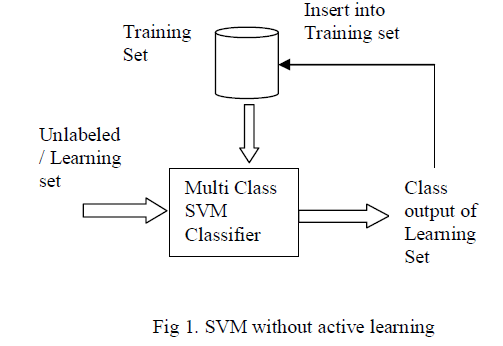The Multi class SVM classifier [1] is trained using a set of initial training samples which is labeled by the user. After training SVM classifier, a set of unlabeled or learning set is given as input to the Multi class SVM classifier and based on the training set, it classifies the input data and the final class information of the input image is obtained. The data related to that particular image is then removed from the learning set and is inserted into the training set along with the class information.

In multiclass SVM, the training set, class information of the training image and the details of the learning image are taken as input. This multiclass SVM classifier can able to classify images only if they have more than two classes. The classifier first finds out the number of classes in the training sequence and then they normalize the class information in to two groups i.e. first class is represented as binary 1 and all the remaining class are considered as binary 0. Then the SVM classifier acts as binary classifier and trains them. Based on the training, it classifies the test or learning image into one of the two groups.

This process gets continued by omitting the class which is considered as 1 and taking remaining class information. Again the above process gets repeated. The process ends at the stage where all the classes are considered for classification process. The details of the image along with the output of the classifier i.e. class information of the learning image is added to the training database so that it can be useful for further classification problems.

IV. SVM WITH ACTIVE LEARNING

To incorporate active learning approach in machine learning, we need to enhance the process of training sample collection. The success of this active learning approach lies in how well the training sample is collected. The ranking procedure is introduced which will find the sample which will best classify the image for a particular class. It is ranked high. The process will continue by ranking all the training samples in the training set. The sample which will be less useful for classification is omitted in inclusion from the training set preparation.

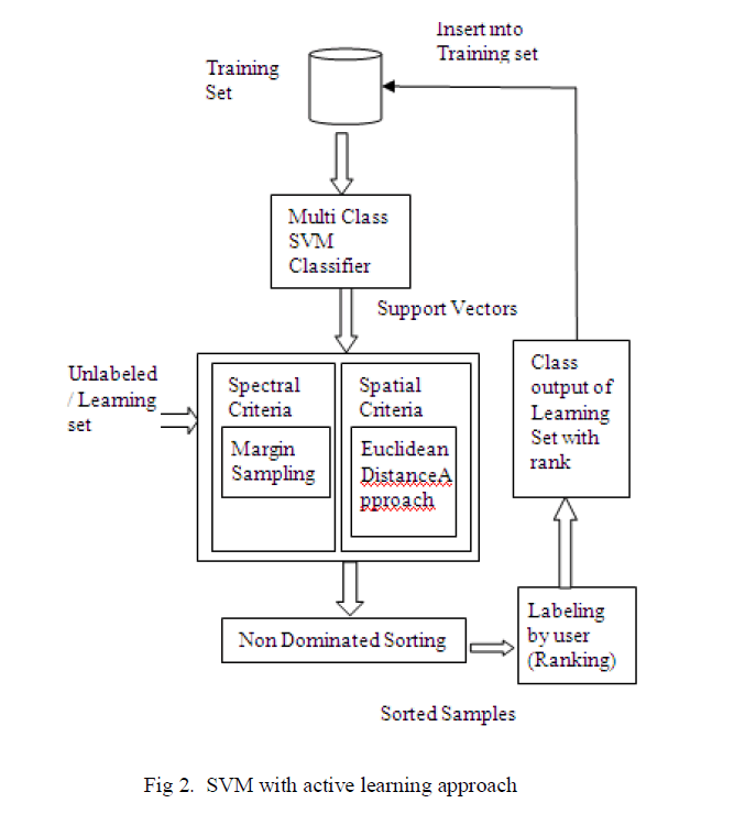
Due to this property, an image can be very well classified to particular class without any ambiguity. Also here two features of the image are considered for classification namely spectral and spatial features. Separate algorithms for each feature are implemented. The overall classification process is depicted in figure 2.

The classifier is trained with initial training set. The classifier generates support vector for the image. By using the support vector, Margin Sampling algorithm for spectral criteria and Euclidean distance approach for spatial criteria are developed. The outputs from both the algorithms are fed to a sorting technique called Non – dominated sorting and the output class information for the training sample is obtained. Then the rank value is obtained from the user as input and all the image detail, class information and the rank value is inserted into the training sample so that they can be considered for further classification.

A. SPECTRAL CRITERIA

Spectral features are the color details of an image. Here we utilize the existing method namely, Margin sampling which have been proved as one of the best method in remote sensing field. Initial training set is prepared by considering RGB, HSV etc.

MARGIN SAMPLING:

This method mainly adopted for classification process in SVM. It is about considering the samples closest to the decision or separating hyperplane. These samples will form the most effective samples which can be used for further classification process.

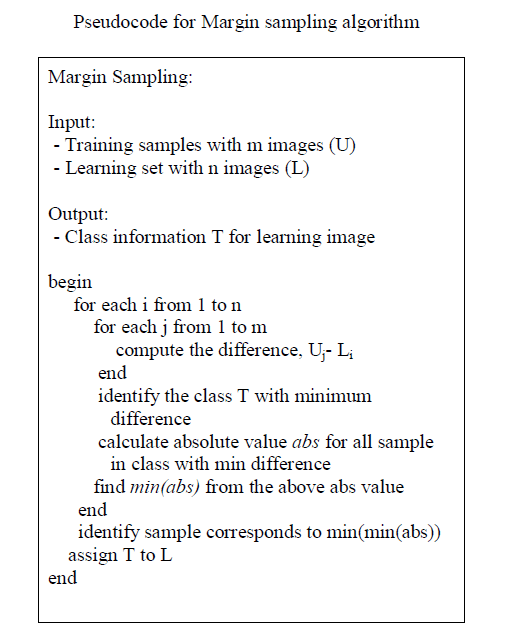
Let S be the initial training set comprises of a samples, U be the unlabeled set comprises of b samples such that b>>a, and T is set of m samples considered for each iteration i.e. T ∈ U. Let there be n different classes identified by the classifier. The classifier is trained with S samples. To classify each sample in T, the margin sampling algorithm works as follows. For each sample ti (i= a+1, a+2, . . , a+m) in T, the number of votes for each class V i.e (vj,1, vj,2 ,...vj,n) is calculated. The class which has the maximum number of votes for the image is selected. Then the absolute value of the class is found and the class which has the minimum absolute value will be considered as the class of that particular image in learning set. The class value for the particular image is the one which has the highest number of votes which will have the minimum of all the absolute values. Thus the image is classified based on spectral criteria.

B. SPATIAL CRITERIA

By considering spatial criteria for image classification, the accuracy of classification can be improved. The spatial factors of an image are texture, shape, color histogram etc. Here the initial training set for the spatial classification is based on color histogram, edge detection and finding co-occurrence matrix.

EUCLIDEAN DISTANCE METHOD:

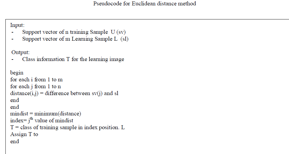
In this method the spatial distance between the training samples and the learning sample is calculated. The support vector from the SVM classifier is obtained. The distance from the support vector sn of the learning image to each of the support vector sj of the training samples are found. Let D = (d1j, d2j…dmj) be the distances where j refers to the learning sample and m refers to the number of samples in the training set. Among the calculated distance, the minimum one is chosen. The minimum distance implies that the learning sample and the training sample are close to each other. So there is more possibility of the learning image to fall in the class of the training image. The class value of the training image is assigned to the learning sample.

V. NON DOMINATED SORTING

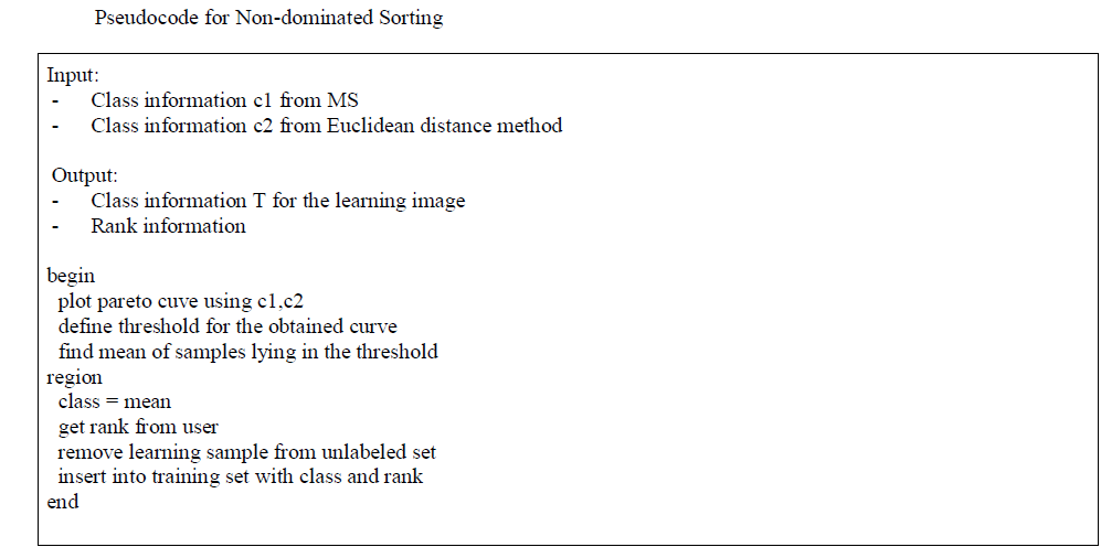
At this stage, we have two outputs, one from spectral criteria c1 and other from spatial criteria c2. The final class information of the sample can be obtained by using non-dominated sorting. The outputs from the two classifiers will serve as input to this sorting. The main objective of non dominated sorting is to select one input such that it satisfies both the criteria under consideration.

The Pareto curve is drawn by plotting the values of the factors considered along XY axis. A threshold is defined. The solution which lies inside this threshold will be considered and the average of the solutions in the selected region is taken as the final outcome of this sorting process.

In our discussion, we consider the class and rank as the two criteria. Consider rank along X axis and class along Y axis. Plot the points from the output of the two classifiers. From the graph obtained, a threshold value is declared and the solution can be derived.

After sorting, the result obtained will be the final class information of the learning sample. The rank information about the sample is obtained from the user and the details about the sample is removed from the learning set and are inserted to the training set along with the rank information so that they can serve for further classification.

VI. DATASET DESCRIPTION

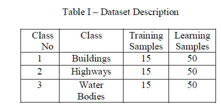
The dataset used for this classification process are the VHR remote sensing images obtained by the QuickBird Satellite. It has a resolution of 0.6m. The images are obtained from the QuickBird imagery.

The classes considered for our discussion are shown in the table.

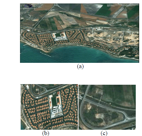Fig 3 - (a) Sample Satellite Image, (b),(c) – Segmented Image used for training, learning process.

The satellite images are segmented to smaller parts and are used for classification process. Fig 3 shows sample satellite images and their segmented parts.

VII. EXPERIMENTAL RESULTS

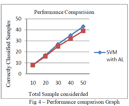
The experiments are conductedusing the training and the learning set. For each iteration, 10 samples from the learning set are taken and are classified and inserted into the training sample set. The number of samples taken for classification and the one which is classified correctly is measured. The graph is drawn using the measured value. The graph (Fig: 4) shows the performance improvement in SVM classifier while using active learning than the one without active learning.

VIII. CONCLUSION

In this paper, a new active learning approach in combination with machine learning approach is used for image classification. Also the consideration of spatial feature in addition to the spectral criteria helps to increase the accuracy of the classifier. This had showed an improvement in the performance of the classifier. SVM is one of the models used in machine learning. Experiments are conducted using VHR images of the QuickBird satellite. Two different classifiers one is SVM without using active learning and other is to use active learning was constructed. Same data were passed over the two classifier and the results were compared. Graph was drawn to show the performance improvement. In addition, to prove the strength of active learning in more depth, we can also use this active learning approach with other models of machine learning like Extended Learning machine, etc as a future work of this paper.

References

E.Pasolli,F.Melgani, D.Tuia,F.Pacifici,and W.J.Emery, “SVM Active Learning Approach for Image Classification Using Spatial Information,” IEEE Transactions on Geoscience and Remote Sensing, (Article in Press)
P. Mitra, B. Uma Shankar, and S. Pal, “Segmentation of multispectral remote sensing images using active support vector machines,” Pattern Recognit. Lett., vol. 25, no. 9, pp. 1067–1074, Jul. 2004.
D. Tuia, F. Ratle, F. Pacifici, M. Kanevski, and W. Emery, “Activelearning methods for remote sensing image classification,” IEEE Trans.Geosci. Remote Sens., vol. 47, no. 7, pp. 2218–2232, Jul. 2009.
S. Rajan, J. Ghosh, and M. Crawford, “An active learning approach tohyperspectral data classification,” IEEE Trans. Geosci. Remote Sens.,vol. 46, no. 4, pp. 1231–1242, Apr. 2008.
T. Luo, K. Kramer, D. B. Golgof, L. O. Hall, S. Samson, A. Remsen, andT. Hopkins, “Active learning to recognize multiple types of plankton,”J. Mach. Learn. Res., vol. 6, no. 4, pp. 589–613, 2005.
J. Muñoz-Marí, D. Tuia, and G. Camps-Valls, “Semisupervised classification of remote sensing images with active queries,” IEEE Trans.Geosci. Remote Sens., vol. 50, no. 10, pp. 3751–3763, Oct. 2012.