International Journal of Innovative Research in Computer and Communication Engineering
ISSN ONLINE(2320-9801) PRINT (2320-9798)
ISSN ONLINE(2320-9801) PRINT (2320-9798)
S.B.Mohan1, A.Rajasekar 2, Dr.T.A.Raghavendiran 3
|
| Related article at Pubmed, Scholar Google |
Visit for more related articles at International Journal of Innovative Research in Computer and Communication Engineering
In this paper an Image Denoising methods and its various parameters are studied. The probability density function of Denoising process is observed by using non-negative Lebesgue-integrable function, cumulative distribution functions and probability mass function are also observed. Edge process control is used for performing denoise signal and it was compared with EQ model. Edge parameter estimation and edge subtraction from the high frequency subband data are analysed.
Keywords |
| Image Denoising – Methods of Denoising; Probability Density Function; Edge Process Model |
INTRODUCTION |
| Image denoising has originated rehabilitated interest among both researchers and camera manufacturers. Faster secure speeds and higher density of image sensors (pixels) result in higher levels of noise in the captured image, which must then be processed by denoising algorithms to yield an image of acceptable quality. This is especially true when images are captured in unfavorable lighting conditions. The goal of such image denoising algorithms is to reduce noise artifacts, at the same time retaining details such as edges and texture in the image. |
| A probability density function (pdf), or density of a continuous random variable, is a function that describes the relative likelihood for this random variable to take on a given value. The probability of the random variable falling within a particular range of values is given by the integral of this variable’s density over that range that is, it is given by the area under the density function but above the horizontal axis and between the lowest and greatest values of the range. The probability density function is nonnegative everywhere, and its integral over the entire space is equal to one. |
| The bounds formulation in [1] showed that the denoising bound is a function of the corrupting noise characteristics (strength and density function) as well as the complexity of the underlying geometric structure of the image patches. Further, the bound is also a function of the amount of redundancy that exists among image patches. In computing the bounds for denoising, we estimated these factors from the underlying noise-free image. As a result, the bounds computation method in [1] cannot be directly applied to the case when only the noisy observation is available. |
II. IMAGE DENOISING |
| As a result of different factors during acquisition and transmission, an image might be degraded by noise leading to a significant reduction of its quality. The artifacts arising due to imperfectness of these processes create obstacles to the perception of visual information by an observer. Thus, for image quality improvement, efficient denoising technique should be applied to compensate such annoying effects. |
| Existing models of image statistics are rooted in the television engineering of the 1950s[2], which relied on a characterization of the auto covariance function for purposes of optimal signal representation and transmission. This work, and nearly all work since, assumes that image statistics are spatially homogeneous (i.e., strict-sense stationary). Another common assumption in image modeling is that the statistics are invariant, when suitably normalized, to changes in spatial scale. The translation- and scale-invariance assumption, coupled with an assumption of Gaussianity, provides the baseline model found throughout the engineering literature: images are samples of a Gaussian random field, with variance falling as f −γ in the frequency domain. In the context of de- noising, if one assumes the noise is additive and independent of the signal, and is also a Gaussian sample, then the optimal estimator is linear. |
A. Denoising Methods |
| The efficient image denoising methods still is a valid challenge, at the crossing of functional analysis and statistics. In spite of the sophistication of the recently proposed methods, most algorithms have not yet attained a desirable level of applicability. All show an outstanding performance when the image model corresponds to the algorithm assumptions, but fail in general and create artifacts or remove image fine structures. The main focus of this paper is, first, to define a general mathematical and experimental methodology to compare and classify classical image denoising algorithms, second, to propose an algorithm (Non Local Means) addressing the preservation of structure in a digital image. The mathematical analysis is based on the analysis of the “method noise”, defined as the difference between a digital image and its denoised version. |
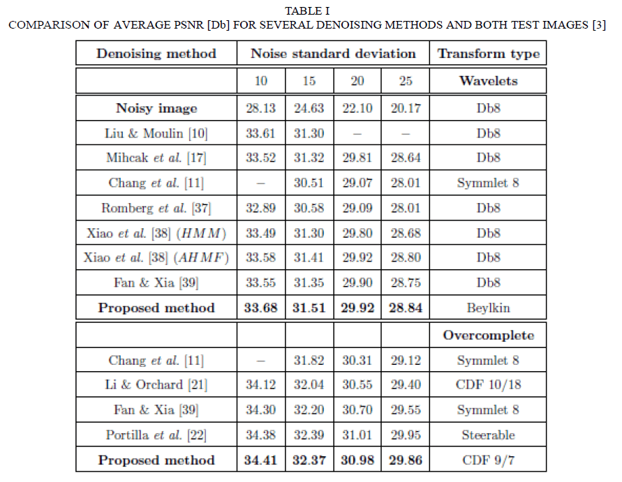
| The proper sampling space is again formed based on the denoised lowpass subband geometrical image prior information, using the proposed quantization based segmentation (except for the subbands from the fourth decomposition level). A complete sampling space dimensionality |M |=15×15 was found to be optimal from the output image PSNR point of view. To verify the performance of the developed algorithms, we applied them to a set of twelve 8 bit 512×512 test images for 100, 225, 400, 625 noise variances of the AWGN. Due to the fact that only two standard test images Lena and Barbara are used for experimental validation of the most of existing Bayesian denoising algorithms, for the fair comparison purpose, only results for these images are presented in this paper and compared with the best Bayesian denoising techniques. Due to the fact that none of the candidates is simultaneously the best for the case of two test images, the benchmarking was performed using the average PSNR for these images for a particular noise variance value (Table 1)[3]. The average PSNR results prove that for the critically sampled transform the performance of the proposed algorithm is the best among known Bayesian techniques, but for the case of the overcomplete domain the method proposed in [4] provides better results. |
 |
| In order to complete experimental validation of the developed algorithms, denoising results obtained using these techniques versus those one presented in [5] and [4] are given in Figure 1 for visual quality comparison. |
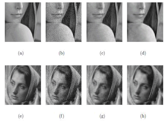 |
| Fig. 1. Experimental results: (a) and (e) fragments of original test images; (b) and (f ) the same fragments corrupted by zero-mean AWGN; ( c ) a n d ( g ) DWT domain denoising results; (d) and (h) DOT domain denoising results.[3] |
| The denoising performance, edge process model is necessary to take into account local data relationships in the stochastic image model. Since this could lead to an increase in computational complexity of the algorithm [3]. |
B. Probability Density Function |
| A probability density function is most commonly associated with absolutely continuous univariate distributions. A random variable X has density fX, where fX is a non-negative Lebesgue-integrable function, if: |
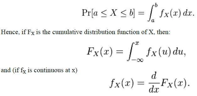 |
| Intuitively, one can think of fX(x) dx as being the probability of X falling within the infinitesimal interval [x, x + dx]. A random variable X with values in a measurable space (X,A) (usually Rn with the Borel sets as measurable subsets) has as probability distribution the measure X∗P on (X,A) : the density of X with respect to a reference measure μ on (X,A) is the Radon–Nikodym derivative: |
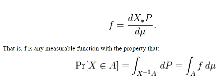 |
| for any measurable set A Σ A . |
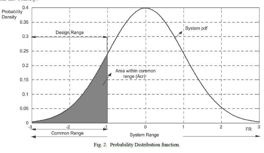
| The terms "probability distribution functions" (Fig. 2) and "probability function" have also sometimes been used to denote the probability density function. However, this use is not standard among probability and statisticians. In other sources, "probability distribution function" may be used when the probability distribution is defined as a function over general sets of values, or it may refer to the cumulative distribution function, or it may be a probability mass function rather than the density. |
 |
III. EDGE PROCESS CONTROL |
| The denoising performance, edge process control is necessary to take into account local data relationships in the stochastic image model. Since this could lead to an increase in computational complexity of the algorithm [3]. |
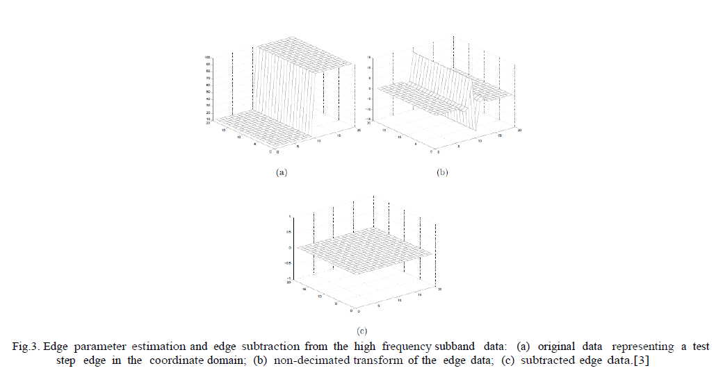
| The residual correlation of the data in the high frequency subbands exists because no linear transform is able to completely decorrelate the edges of real images. This phenomenon is illustrated in Figure 10 where a simple example of step edge (Figure 3, a) is transformed using non-decimated wavelet trans- formation (Figure 3,b). Therefore, if one finds a way to completely “remove” the edges from the subband data, this will allow an increase in performance by providing additional decorrelation (Figure 3,c). |
| Our goal is to introduce the edge process model (EP) and to compare it with the EQ model. The EQ model belongs to the class of intraband stochastic image models and assumes that the wavelet coefficients are Gaussian (in the original paper of Lopresto et al. the Generalized Gaussian [6]) distributed, with zero mean and variances that depend on the coefficient location within each subband. It is also assumed that the variance is slowly varying. |
 |
IV. CONCLUSION |
| In this paper we have analysed the theory of image denoising. Aiming at enhancing denoising performance without increasing algorithmic computational complexity, the edge process stochastic image model was proposed as a way to decrease the residual correlation in the high frequency subbands. In this case the significant gain in the PSNR was obtained for all tested AWGN variances. As it was mentioned, the main open issue of the EP model is the reliable estimation of the model parameters in the presence of noise. Therefore, we will concentrate on the solution to this problem in our ongoing research, and will exploit it for other applications such as image compression [7] and watermarking [8] where attacks and watermark are power limited due to perceptual constraints on image fidelity. |
References |
|