International Journal of Advanced Research in Electrical, Electronics and Instrumentation Engineering
ISSN ONLINE(2278-8875) PRINT (2320-3765)
ISSN ONLINE(2278-8875) PRINT (2320-3765)
Ahmad Shakeeb1, Bhawesh Kr Bharti2, Arvind kumar3, Bimlesh Prasad4, Prof. L.Ramesh5
|
| Related article at Pubmed, Scholar Google |
Visit for more related articles at International Journal of Advanced Research in Electrical, Electronics and Instrumentation Engineering
Improvement of STLF has been a cause of concern right since the origin of Load Forecasting for making numerous number of decision making process. The financial impact of an electrical blackout is very profound to both suppliers and consumers. A multiagent system for electric load forecasting, especially suited to simulating the different social dynamics involved in distribution systems, is presented. We also present here a combined aggregative short-term load forecasting method for smart grids, a novel methodology that allows us to obtain a global prognosis by summing up the forecasts on the compounding individual loads. In this paper a simple model is taken to estimate the relationship between demand and the driver’s variable. The results of various types STLF are taken and errors are calculated. After conclusion
INTRODUCTION |
| SOLVING the short-term forecasting problem is essential in the decision-making process of any electric utility. During the last two decades, a wide variety of methods have been proposed due to the importance of STLF. In those the effective methods are less ones. The parameters of load forecasting were first linearly varied in which the desired could not be obtained. Now the real parameters are varied non-linearly which give forecasting has fuzzy logic approaches and neural network based approaches. |
| Both NN and FLSs are universal approximators with the capability of identifying and approximating nonlinear relationships between independent (inputs) and dependent (missions) variables to any arbitrary degree of accuracy. The popularity of these models for prediction is due to their universal approximation capability, the excellent learning capabilities of NNs, and FLS capability in simultaneous handling of quantitative/qualitative information and uncertainties. These two model types represent the best alternatives for modeling, prediction, and forecasting purposes as it can adapt to any type conditions. |
| When we coin the word intelligent we mean the effective methods of artificial intelligence in the field of load forecasting. When we use the tools of intelligence such as Fuzzy logic, Neural networks, Petri nets and evolution algorithm in designing load forecasting control ,then historically this field has been known as intelligent load forecasting. |
| There are three aspects of intelligence that are : |
| i. Intelligent Observe – Data Analysis |
| ii. Intelligent Prediction – system identification |
| iii. Intelligent Interaction – Adaptive Control |
| When we design any non-linear or linear technique we have to be concern with model uncertainties (derived from mathematical models), system adaptively to change with variables and its distribution in nature. |
| Coming to Load Forecasting, first we define Load: Load is generic term for something in the circuit that will draw power which can vary widely. The system load is a random non-stationary process composed of thousands of individual components. The system load behavior is influenced by a number of factors, which can be classified as: economic factors, time, day, season, weather and random effects. Load Forecasting can be thought of as the set of processes, activities, and toolsets used to create predictions to support operational decision making of various loads. |
| To predict Load Forecasting we use tools like Load Curve and Load Characteristics. Like we have collected a data TNEB (Tamil Nadu Electricity Board) for Chengalpattu for a day power consumption. The Daily Load Curve is as follows: |
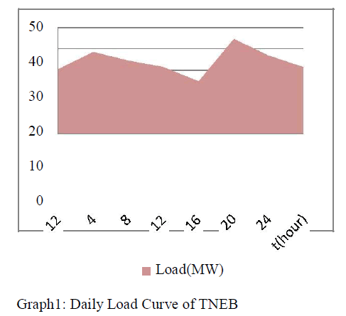 |
| The Load Curve gives the information of load on the power station during different running hours or day or months , the maximum demand (peak of the curve),Energy produced (area under the curve), load factor and average loading. |
| The Typical seasonal workday TNEB Load Profile is as follows: |
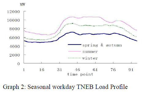 |
MATHEMATICAL MODELLING |
| The behavior of time series or a process in the past and its mathematical modeling so that the future can be extracted from it. The typical curves used in power system forecasting are: |
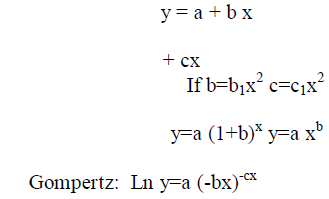 |
| The coefficients used above are nothing regression coefficients. In most cases, linear dependency gives the best results. But in practical situations linearity does not satisfy load behavior. We need to go for non-linear load curves and characteristics for evaluating load forecasting. |
| Basically load forecasting has two broad classifications: |
| i. Statistical Intelligence Methods |
| ii. Artificial Intelligence Methods |
| iii. Data Mining methods |
| Only advanced statistical and artificial intelligence methods are considered which are popular nowadays. |
| Various Statistical Intelligence Methods are: |
| a) Regression Methods |
| b) Times Series |
| Various Artificial Intelligence Methods are: |
| a) Neural Networks Method |
| b) Fuzzy Logic Method |
| c) Knowledge Based Expert System |
| d) Petri nets system |
| Advancement of some popular system are as follows: |
| 1. Regression Methods |
| Mbamalu and El-Hawary (1993) used the following load model for applying this analysis: |
 |
| The data analysis program allows the selection of the polynomial degree of influence of the variables from 1 to5. In most cases, linear dependency gives the best results. Moghram and Rahman (1989) evaluated this model and compared it with other models for a 24-h load forecast. Barakat (1990) used the regression model to data and check seasonal variations. The model developed by Papalexopulos and Hesterberg (1990) produces an initial daily peak forecast and then uses this initial peak forecast to produce initial hourly forecasts. |
| In the next step, it uses the maximum of the initial hourly forecast, the most recent initial peak forecast error, and exponentially smoothed errors as variables in a regression model to produce an adjusted peak forecast. Haida and Muto (1994) presented a regression-based daily peak load forecasting method with a transformation technique. Their method uses a regression model to predict the nominal load and a learning method to predict the residual load. Haida (1998) expanded this model by introducing two trendprocessing techniques designed to reduce errors in transitional seasons. Trend cancellation removes annual growth by subtraction or division, while trend estimation evaluates growth by the variable transformation technique. Varadan and Makram (1996) used a least-squares approach to identify and quantify the different types of load at power lines and substations. Hyde and Hodnett (1997) presented a weather-load model to predict load demand for the Irish electricity supply system. To include the effect of weather, the model was developed using regression analysis of historical load and weather data. Hyde and Hodnett (1997b) later developed an adaptable regression model for 1-day-ahead forecasts, which identities weather-insensitive and -sensitive load components. Linear regression of past data is used to estimate the parameters of the two components. Broadwater et al. (1997) used their new regression-based method, Nonlinear Load Research Estimator (NLRE), to forecast load for four substations in Arkansas, USA. This method predicts load as a function of customer class, month and type of day. Al-Garni (1997) developed a regression model of electric energy consumption in Eastern Saudi Arabia as a function of weather data, solar radiation, population and per capita gross domestic product. Variable selection is carried out using the stepping-regression method, while model adequacy is evaluated by residual analysis. The nonparametric regression model of Charytoniuk (1998) constructs a probability density function of the load and load effecting factors. The model produces the forecast as a conditional expectation of the load given the time, weather and other explanatory variables, such as the average of past actual loads and the size of the neighborhood. Alfares and Nazeeruddin (1999) presented a regression-based daily peak load forecasting method for a whole year including holidays. To forecast load precisely throughout a year, different seasonal factors that effect load differently in different seasons are considered. In the winter season, average wind chill factor is added as an explanatory variable in addition to the explanatory variables used in the summer model. In transitional seasons such as spring and Fall, the transformation technique is used. Finally for holidays, a holiday effect load 24 H. K. Alfares and M. Nazeeruddin is deducted from normal load to estimate the actual holiday load better. |
| After 1999 time series had a major power play to accomplished and regression gave the way auto regression as we needed an intelligent control. Evolution Algorithm was developed by Regression Methods but was not very much successful. |
Preview Results: |
| The C-GRNN was developed with the toolboxes of neural networks from the software MATLAB. The function used was the NEWGRNN. The M-GRNN and the MR-GRNN were developed in MATLAB without the use of the toolboxes of neural networks. All of the systems were trained with the same training dataset, and for all of them, the parameter spread of the conventional and modified GRNNs was chosen using the procedure. For the modified GRNN, the number of samples was set to 50. The procedure to reduce the number of inputs of the GRNN was applied only for the modified GRNN. It was decided to preserve the information about the months and holidays (inputs 1 and 7, respectively), with a minimum of six inputs. Before training the Grams, the local loads of the training dataset were preprocessed using the filter proposed [20]. The parameters of the filter were spread 0.1, tolerance error 30%, and an MAF of three samples. For the global load, the results were obtained only for the PFF for the three different forecasters. For the local loads, the results were obtained for the LLF and PFF for the three different forecasters: C-GRNN, M-GRNN, and MR-GRNN. The MAPE was calculated for the forecasts of conventional days (total of 7 forecasted, 08-01-2009 to 14-01-2009) and the holidays (total of two forecasted, 26-01-2009 and 06- 02-2009). The time spent for each forecaster to forecast one day was measured. The time spent for training the GRNN was very small, considering that it was just memory allocation. |
A. Global Load |
| The MAPEs obtained for the global load forecasting of conventional days and holidays with the forecasters CGRNN, M-GRNN, and MR-GRNN and the average times spent to forecast one day for each global load forecaster, are shown in Table IV. Fig. 4. Global load forecasting. |
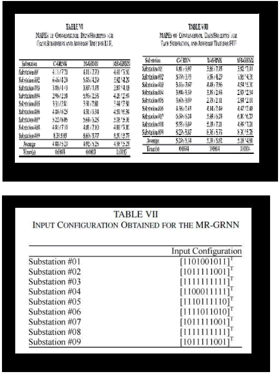
| The input configuration of the MR-GRNN can be seen in Table V, where ones correspond to the active inputs and zeros correspond to the inactive inputs. The global load forecasting can be observed in Fig. 4. In Table IV, the MRGRNN obtained the best results for the conventional day’s forecasts, but for the holidays, the best results were achieved with the C-GRNN and M-GRNN. These results suggest that for the conventional days, it is possible to achieve better results by using M-GRNN and by reducing the number of inputs. For the holidays, it is better to consider all of the ten inputs. In Table IV, it can be observed that the average time spent for one forecaster to forecast one day is very low, less than 0.01. However, it can be noted that M-GRNN, when with C-GRNN, reduces this time by almost six times. The input configuration obtained with the MR-GRNN suggests that the inputs 6, 9, and 10 are not so relevant for the global load forecasting, which means that it is possible to omit the information about the daylight saving time and the values of the maximum and minimum load of the day . |
B. Local Loads |
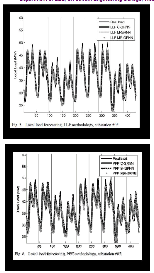
| Local Load Forecaster Methodology: The MAPEs obtained for the local load forecasting of conventional days and holidays, obtained for the LLF methodology with the forecasters C-GRNN, M-GRNN, and MR-GRNN, and the average times spent for one forecaster to forecast one day for each local load forecaster are shown in Table VI. The input configuration of the MR-GRNNs is given in Table VII, where ones correspond to the active inputs and zeros correspond to the inactive inputs. The local load forecasting of substation #03 is given in Fig. 5. For the LLF methodology, better results were achieved with CGRNN, followed by M-GRNN and MR-GRNN. The average time spent for one forecaster to forecast one day also suggests that the M-GRNN is able to provide accurate results faster. |
 |
 |
| The input configurations obtained with the MR-GRNNs suggest that in some cases, it is possible to reduce the number of inputs, and in other cases, this reduction is not advisable (e.g., substations #03 and #08). |
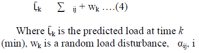
| 2) PFF Methodology: The MAPEs obtained for the local load forecasting of conventional days and holidays, obtained for the PFF methodology with the forecasters CGRNN, M-GRNN, and MR-GRNN, and the average times spent for one forecaster to forecast one day for each local load forecaster are shown in Table VIII. The input configuration of MR-GRNNs is shown in Table IX, where ones correspond to the active inputs, and zeros correspond to the inactive inputs. The local load forecasting of substation #03 is given in Fig. 6. For the PFF methodology, better results were achieved with M-GRNN, followed by MR-GRNN and C-GRNN. The local load in this methodology depends on the global load forecasting and, in this case, it suggests that better results can be achieved by minimizing the global load forecasting errors. The average time spent for one forecaster to forecast one day also suggests that M-GRNN is able to provide accurate results faster. The input configurations obtained with MR-GRNNs suggest that in some cases, it is possible to reduce the number of inputs and, in other cases, this reduction is not advisable (e.g., substations #01, #05, and #08). |
CONCLUSION |
| In this paper, a modification in the C-GRNN was proposed, and a procedure to reduce the number of inputs of the GRNN for STMLF was presented. Tests were carried out with active loads of nine New Zealand electrical substations for two methodologies, namely, the PFF and the LLF, and for three different forecasters, namely, CGRNN, M-GRNN, and MR-GRNN. The M-GRNN was found to have the advantage to maintain the same characteristics of C-GRNN, such as good generalization ability, stability, and training in one presentation of the training dataset, with the ability to provide faster forecasting. The MR-GRNN was found to have the ability to reduce the number of inputs, avoiding redundancies that may compromise the results in some cases. To design the inputs of the neural networks, the previous study of the local loads was not necessary, thus reducing the complexity of the STMLF problem. Results were also obtained by using only the first three months of 2007 and 2008, and the first six months of 2007 and 2008, in the training dataset. The MAPEs obtained were almost the same, indicating that these systems are very robust in terms of the possibility to increase the training dataset without losing stability. In most of the cases, daily peak values were not predicted correctly. It occurs because GRNN estimates are based upon regression, so peak values can sometimes remain lower than they really are. To correct this, it is possible to use preprocessing data and filtering according to what was proposed on [18] and a small gain can also be applied to compensate for this demand. This gain can be calculated from previous loads, or it can also be estimated by a GRNN designed to perform this task. It does not pose a problem at all and it does not limit the usefulness of the model. The studies performed in the New Zealand system loads can be performed in any system; consequently, the applicability is possible in any system since the data are available. The proposed systems are robust and very fast and are able to work in real-time operation. It is considered that future works effectuate STMLF by using other neural networks, especially with the ART family, which has already been done for global load forecasting. |
2. Times Series: |
| Time series methods are based on the assumption that the data have an internal structure, such as autocorrelation, trend or seasonal variation. The methods detect and explore such a structure which relates to basic concepts of Short-term Load Forecasting. |
| Time series have been used for decades in such fields as economics, digital signal processing, as well as electric load forecasting. It has been observed that unique patterns of energy and demand pertaining to fast-growing areas are difficult to analyze and predict by direct application of time-series methods. However, these methods appear to be among the most popular approaches that have been applied and are still being applied to STLF. Using the time-series approach, a model is first developed based on the previous data, and then future load is predicted based on this model. |
| Some of the time series models used for load forecasting are as follows:. |
2.1. Autoregressive (AR) model |
| If the load is assumed to be a linear combination of previous loads, then the autoregressive (AR) model can be used to model the load profile, which is given by Liu (1996) as: |
 |
| =1……m are unknown coefficients, and (4) is the AR model of order m. The unknown coefficients in (4) can be tuned on-line using the well-known least mean square (LMS) algorithm of Mbamalu and El-Hawary (1993). The algorithm presented by El-Keib (1995) includes an adaptive autoregressive modeling technique enhanced with partial autocorrelation analysis. Huang (1997) proposed an autoregressive model with an optimum threshold stratification algorithm. This algorithm determines the minimum number of parameters required to represent the random component, removing subjective judgment, and improving forecast accuracy. Zhao (1997) developed two periodical autoregressive (PAR) models for hourly load forecasting. |
2.2. Autoregressive moving-average (ARMA) model |
| In the ARMA model the current value of the time series y(t) is expressed linearly in terms of its values at previous periods [y(t-1),y(t-2),……..] and in terms of previous values of a white noise[a(t),a(t-1…]. For an ARMA of order (p, q), the model is written as: |
| y(t)= ø1y(t-1)+……+ øpy(t-p)+a(t) - 1a(t-1) - ……… qa(t-q). |
| The parameter identification for a general ARMA model can be done by a recursive scheme, or using a maximumlikelihood approach, which is basically a non-linear regression algorithm. Barakat (1992) presented a new timetemperature methodology for load forecasting. In this method, the original time series of monthly peak demands are decomposed into deterministic and stochastic load components, the latter determined by an ARMA model. Fan and McDonald (1994) used the WRLS (Weighted Recursive Least-Squares) algorithm to update the parameters of their adaptive ARMA model. Chen (1995) used an adaptive ARMA model for load forecasting, in which the available forecast errors are used to update the model. Using minimum mean square error to derive error learning coefficients, the adaptive scheme outperformed conventional ARMA models. |
2.3. Autoregressive integrated moving-average (ARIMA) model |
If the process is non-stationary, then transformation of the series to the stationary form has to be done first. This transformation can be performed by the differencing 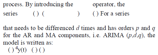 |
| The procedure proposed by Elrazaz and Mazi (1989) used the trend component to forecast the growth in the system load, the weather parameters to forecast the weather sensitive load component, and the ARIMA model to produce the non-weather cyclic component of the weekly peak load. Barakat et al. (1990) used a seasonal ARIMA model on historical data to predict the load with seasonal variations. Juberias (1999) developed a real time load forecasting. ARIMA model that includes the meteorological influence as an explanatory variable. |
2.4 ARMAX Model based on genetic algorithms |
| The genetic algorithm (GA) or evolutionary programming (EP) approach is used to identify the autoregressive moving average with exogenous variable (ARMAX) model for load demand forecasts. By simulating natural evolutionary process, the algorithm offers the capability of converging towards the global extremum of a complex error surface. It is a global search technique that simulates the natural evolution process and constitutes a stochastic optimization algorithm. Since the GA simultaneously evaluates many points in the search space and need not assume the search space is differentiable or unimodal, it is capable of asymptotically converging towards the global optimal solution, and thus can improve the fitting accuracy of the model. The general scheme of the GA process is briefly described here. The integer or real valued variables to be determined in the genetic algorithm are represented as a Ddimensional vector P for which a fitness f(p) is assigned. The initial population of k parent vectors Pi,i=1……,k, is generated from a randomly generated range in each dimension. Each parent vector then generates an offspring by merging (crossover) or modifying (mutation) individuals in the current population. Consequently, 2k new individuals are obtained. Of these, k individuals are selected randomly, with higher probability of choosing those with the best fitness values, to become the new parents for the next generation. This process is repeated until f is not improved or the maximum number of generations is reached. Yang (1996) described the system load model in the following ARMAX form: |
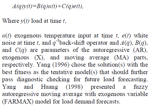 |
| The model is formulated as a combinatorial optimization problem, then solved by a combination of heuristics and evolutionary programming. Ma (1995) used a genetic algorithm with a newly developed knowledge augmented mutation-like operator called the forced mutation. Lee (1997) used genetic algorithms for long-term load forecasting, assuming different functional forms and comparing results with regression. |
SIMULATION RESULTS |
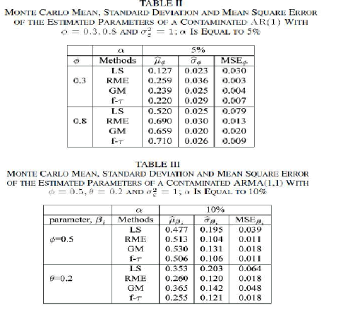 |
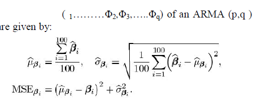
| Before studying the practical case of load forecasting, let us first apply the proposed RME method on synthetic processes in order to compare it with the Generalized Mestimates and the filtered -estimates. The GM estimates are chosen because of their wide use in power systems. In the statistical literature, the filtered -estimates are newly developed robust estimators for ARMA models. They offer a high breakdown point of 50% with a high efficiency of 0.95. They are proposed in the Book of Maronna et al. [3]. Maronna et al. recommend their use since they insure a good tradeoff between robustness and efficiency under normality. We study the impact of the outliers on parameter estimation. The mean, standard deviation and mean squared error of the parameters are computed using Monte Carlo simulations and given in Tables II–III. The Monte Carlo consists in generating 100 AR(1) and ARMA (1,1) processes of length 1000 with different noises. The noises follow a Gaussian distribution(0,1). The positions of outliers are chosen randomly. The percentage of outliers is denoted by . The mean, standard deviation and the mean squared error of the estimated parameters |
 |
| Table II illustrates the results obtained with two autoregressive models . The outliers are generated from a point mass at 4. The table shows the robustness of the RME. The RME performs best for Φ=0.3 . At Φ=0.8, the filtered are slightly better than the RME. Table III is obtained using outliers generated from a Gaussian i.i.d. process N(0,4) . In this case, the outliers are not very large and contained in the bulk of the data. This means a certain difficulty to detect them by three-sigma rule. From Table III, we conclude that the RME-based estimator and filtered estimator have the same performance and are the best estimators since they have the smallest mean squared errors (MSE). However, we prefer the RME to the filtered due to its simplicity and short time execution. The relative computing times of the RME and filtered are respectively 1 and 2. The RME is a quicker executing method than the filtered . The algorithm previously defined is also much easier to program than the algorithm of the filtered [3]. The GM is better than the LS (least squares estimator) which is natural since the LS is not robust. |
APPLICATION TO LOAD TIME SERIES FORECASTING |
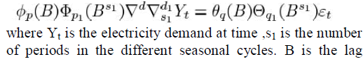
| This section is devoted to the study of a practical case to show the effectiveness of the proposed method. In this case, it has the advantage of simplicity, robustness and fast execution and is implemented to online estimation and forecasting purposes. Forecasting load time series using SARIMA models is extensively used in the literature [13], [14]. RTE, the transmission operator that manages and operates the French electric power transmission system, is confronted to the presence of outliers in the French daily electric consumptions. RTE uses a SARIMA model in its daily forecasting. The series exhibit a trend and several major cycles (daily, weekly, seasonal, yearly, etc.). One of the figure illustrates the load demand from Saturday July2, 2005 to Monday July 25, 2005. Since July 14 is a national holiday to mark the anniversary of the storming of the Bastille, there is a break appearing on Thursday 14 and Friday 15 [approximately from observation 600 to 700]. The dataset consists of intraday half-hourly load series from February 1, 2004 to June 14, 2005. We consider the 48 series corresponding to the load demand at different hours . Each series has 600 observations. 500 being used for estimating the model and 100 for out-of-sample evaluation. Another figure displays the one-week differentiated load time seriesat 07:00 in 2005, which is given by for , where is the consumption of the day at 07:00.We notice the presence of spikes at some sampling times, which are represented by circles in the figure. Called breaks or outliers in statistics, these spikes stem from the abrupt changes in the differentiated load series from one day to the other over one week. Online records and archives of total power consumption in metropolitan France (excluding Corsica) is provided by RTE [15]. The data used can be downloaded online. The load time series is first corrected from the influence of the weather by using a regression model where the exploratory variables are the temperature and the nebulosity. Then an ARIMA model is fitted to the residuals. A seasonal ARIMA model, SARIMA(p,d,q) (p1,d1,q1)follow the equation: |
 |
| operator. |
| The maximum-likelihood-based classical approach applied after deleting the unusual observations by the “three-sigma” rejection rule, is denoted by CM. The “threesigma” rule consists in rejecting observations that are outlying beyond three times the robustly estimated standard deviation from a robust estimate of the trend (that is, the central part) of the time series. The load series at night hours such as 02:00 is not contaminated by non-working days or other events happening in the day. The curves confirm the high efficiency of the RME-based and the filtered estimates which has the same performance as the CM. The performances vary then with the series. This is quite normal since some hours are more contaminated than others. In Fig. 7(a), we plot the quantiles |
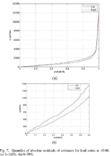 |
| of the absolute values of the residuals in the RME and CM methods for the series at 10:00. Fig. 7(b) zooms in the quantiles less than 0.7. It is seen that the RME-based estimate yields the smallest quantiles, and hence gives the best fit to the bulk of data. We remark that a small fraction of residuals obtained with the RME-based estimator are very large. These residuals correspond to the outliers. |
3.a. Neural Networks Method: |
| The use of artificial neural networks (ANN or simply NN) has been a widely studied load forecasting technique since 1990 . Neural networks are essentially non-linear circuits that have the demonstrated capability to do non-linear curve fitting. |
| The outputs of an artificial neural network are some linear or non-linear mathematical function of its inputs. The inputs may be the outputs of other network elements as well as actual network inputs. In practice network elements are arranged in a relatively small number of connected layers of elements between network inputs and outputs. Feedback paths are sometimes used. |
| In applying a neural network to load forecasting, one must select one of a number of architectures (e.g. Hopfield, back propagation, Boltzmann machine), the number and connectivity of layers and elements, use of bi-directional or uni-directional links and the number format (e.g. binary or continuous) to be used by inputs and outputs. |
| The most popular artificial neural network architecture for load forecasting is back propagation. This network uses continuously valued functions and supervised learning. That is, under supervised learning, the actual numerical weights assigned to element inputs are determined by matching historical data (such as time and weather) to desired outputs (such as historical loads) in a preoperational “training session”. Artificial neural networks with unsupervised learning do not require pre-operational training. |
| Bakirtzis developed an ANN based short-term load forecasting model for the Energy Control Center of the Greek Public Power Corporation. In the development they used a fully connected three-layer feed forward ANN and a back propagation algorithm was used for training. Input variables include historical hourly load data, temperature, and the day of week. The model can forecast load profiles from one to seven days. Also Papalexopoulos developed and implemented a multi-layered feed forward ANN for short-term system load forecasting. In the model threeBakirtzis developed an ANN based short-term load forecasting model for the Energy Control Center of the Greek Public Power Corporation. In the development they used a fully connected three-layer feed forward ANN and a back propagation algorithm was used for training. Input variables include historical hourly load data, temperature, and the day of week. The model can forecast load profiles from one to seven days. Also Papalexopoulos developed and implemented a multi-layered feed forward ANN for short-term system load forecasting. In the model three types of variables are used as inputs to the neural networks: seasonal related inputs, weather related inputs, and historical loads. Khotanzad described a load forecasting system known as ANNSTLF. It is based on multiple ANN strategy that captures various trends in the data. In the development they used a multilayer perceptron trained with an error back propagation algorithm. ANNSTLF can consider the effect of temperature and relative humidity on the load. It also contains forecasters that can generate the hourly temperature and relative humidity forecasts needed by the system. An improvement of the above system was described in one of the paper. |
| In the new generation, ANNSTLF includes two ANN forecasters: one predicts the base load and the other forecasts the change in load. The final forecast is computed by adaptive combination of these forecasts. The effect of humidity and wind speed are considered through a linear transformation of temperature. At the time it was reported , ANNSTLF was being used by 35 utilities across the USA and Canada. Chen also developed a three layer fully connected feed forward neural network and a back propagation algorithm was used as the training method. Their ANN though considers electricity price as one of the main characteristics of the system load. Many published studies use artificial neural networks in conjunction with other forecasting techniques such as time series and fuzzy logic. |
3.b.Fuzzy logic |
| It is well known that a fuzzy logic system with centroid defuzzification can identify and approximate any unknown dynamic system ( load in this case) on the compact set to arbitrary accuracy. Liu (1996) observed that a fuzzy logic system has great capability in drawing similarities from huge data. The similarities in input data (L –I -- L0) can be identified by different first-order differences (Vk) and second-order differences (Ak), which are defined as: |
| The fuzzy logic-based forecaster works in two stages: training and on-line forecasting. In the training stages, the metered historical load data are used to train a 2m-input, 2n-output fuzzy-logic based forecaster to generate patterns database and a fuzzy rule base by using first and secondorder differences of the data. After enough training, it will be linked with a controller to predict the load change online. If a most probably matching pattern with the highest possibility is found, then an output pattern will be generated through a centroid defuzzifier. |
| Several techniques have been developed to represent load models by fuzzy conditional statements. Hsu (1992) presented an expert system using fuzzy set theory for STLF. The expert system was used to do the updating function. Short-term forecasting was performed and evaluated on the Taiwan power system. Later, Liang and Hsu (1994) formulated a fuzzy linear programming model of the electric generation scheduling problem, representing uncertainties in forecast and input data using fuzzy set notation. Al-Anbuky (1995) discussed the implementation of a fuzzy-logic approach to provide a structural framework for the representation, manipulation and utilization of data and information concerning the prediction of power commitments. Neural networks are used to accommodate and manipulate the large amount of sensor data. |
| Srinivasan (1992) used the hybrid fuzzy-neural technique to forecast load. This technique combines the neural network modeling and techniques from fuzzy logic and fuzzy set theory. The models were later enhanced by Dash (1995). This hybrid approach can accurately forecast on weekdays, public holidays, and days before and after public holidays. Based on the work of Srinivasan , Dash (1995) presented two fuzzy neural network (NN) models capable of fuzzy classification of patterns. The first network uses the membership values of the linguistic properties of the past load and weather parameters , where the output of the network is defined as the fuzzy class membership values of the forecasted load. The second network is based on the fact that any expert system can be represented as a feed forward NN. Mori and Kobayashi (1996) used fuzzy inference methods to develop a non-linear optimization model of STLF, whose objective is to minimize model errors. The search for the optimum solution is performed by simulated annealing and the steepest descent method. Dash (1996) used a hybrid scheme combining fuzzy logic with both neural networks and expert systems for load forecasting. Fuzzy load values are inputs to the neural network, and the output is corrected by a fuzzy rule inference mechanism. Ramirez-Rosado and Dominguez- Navarro (1996) formulated a fuzzy model of the optimal planning problem of electric energy. Computer tests indicated that this approach outperforms classical deterministic models because it is able to represent the intrinsic uncertainty of the process. Chow and Tram (1997) presented a fuzzy logic methodology for combining information used in spatial load forecasting, which predicts both the magnitudes and locations of future electric loads. The load growth in different locations depends on multiple, conflicting factors, such as distance to highway, distance to electric poles, and costs. Therefore, Chow (1998) applied a fuzzy, multi-objective model to spatial load forecasting. The fuzzy logic approach proposed by Senjyu (1998) for next-day load forecasting offers three advantages. These are namely the ability to |
| (1) handle non-linear curves, |
| (2) forecast irrespective of day type and |
| (3) provide accurate forecasts in hard-to-model situations. |
| Mori (1999) presented a fuzzy inference model for STLF in power systems. Their method uses tabu search with supervised learning to optimize the inference structure (i.e. number and location of fuzzy membership functions) to minimize forecast errors. Wu and Lu (1999) proposed an alternative to the traditional trial and error method for determining of fuzzy membership functions. An automatic model identification is used, that utilizes analysis of variance, cluster estimation, and recursive least squares. Mastorocostas (1999) applied a two-phase STLF methodology that also uses orthogonal least-squares (OSL) in fuzzy model identification. Padma kumari (1999) combined fuzzy logic with neural networks in a technique that reduces both errors and computational time. Srinivasan (1999) combined three techniques-fuzzy logic, neural networks and expert systems in a highly automated hybrid STLF approach with unsupervised learning. |
SIMULATION RESULTS: |
1) Number of Configurations to be Evaluated by the SRA: |
| Table V shows the dimension of the solution space corresponding to different dimensions of the correlation mask and considering depths of 25, 49, and 73. |
2) Hypothesis for STLF With FIR and SRA: |
| 1) The FIR methodology proposed by Cellier uses 5-NN in the fuzzy forecast. In this paper, different values for the parameter -NN (4-6) were used. |
| 2) The “α ” value (coefficient of elasticity) from the SRA algorithm was taken as 0.92 |
| The minimum error of training and testing was obtained using k=4, using the configuration V8 and a depth of 25. |
 |
 |
3.c. Knowledge Based Expert System |
| Rule based forecasting makes use of rules, which are often heuristic in nature, to do accurate forecasting. Expert systems, incorporates rules and procedures used by human experts in the field of interest into software that is then able to automatically make forecasts without human assistance. |
| Expert system use began in the 1960’s for such applications as geological prospecting and computer design. Expert systems work best when a human expert is available to work with software developers for a considerable amount of time in imparting the expert’s knowledge to the expert system software. Also, an expert’s knowledge must be appropriate for codification into software rules (i.e. the expert must be able to explain his/her decision process to programmers). An expert system may codify up to hundreds or thousands of production rules. Ho proposed a knowledge-based expert system for the short term load forecasting of the Taiwan power system. Operator’s knowledge and the hourly observations of system load over the past five years were employed to establish eleven day types. Weather parameters were also considered. The developed algorithm performed better compared to the conventional Box- Jenkins method. Rahman and Hazim developed a siteindependent technique for short-term load forecasting. Knowledge about the load and the factors affecting it are extracted and represented in a parameterized rule base. This rule base is complemented by a parameter database that varies from site to site. The technique was tested in several sites in the United States with low forecasting errors. The load model, the rules, and the parameters presented in the paper have been designed using no specific knowledge about any particular site. The results can be improved if operators at a particular site are consulted. |
3.d. Petri nets system |
| PN models can be readily used to describe a combined system model of several interacting subsystems . Each subsystem may interact with the other subsystem via token exchange. In the dispatch model that we’ll develop , we divided the model into three parts : the ISO , the GENCOS and the LSE’s. |
| GENCOS & LSEs submit generation bids & load bids to the ISO, which then dispatches the bids according to the merit lists set by the price priority of the bids. The ISO model is supposed to be a deterministic one, as all the information is available to the ISO, such as the amount of supply & the amount of load and Transmission line capacities. The GENCOS MODEL and LSEs model are stochastic to simulate the uncertainties in their decision making process. The models interact with each other by exchanging tokens. |
| PN Models are able to describe “what – if” situations. For example, in strategic bidding, A Generator owner may ask himself questions such as” if others bid high(low) in a peak load time period, what are my bids?” or “what if the real time load is lower than the forecasted load?” Petri nets models can simulate such kind of situations and provide an answer to these “what if” Questions. |
| Petri nets are widely used in the simulation of discrete event system because the decision- making system in a bid – based energy market is a discrete system that accommodates independent bidders and require a bid based priority dispatch , using Petri nets to describe the information is appropriate . |
RESULTS AND DISCUSSION |
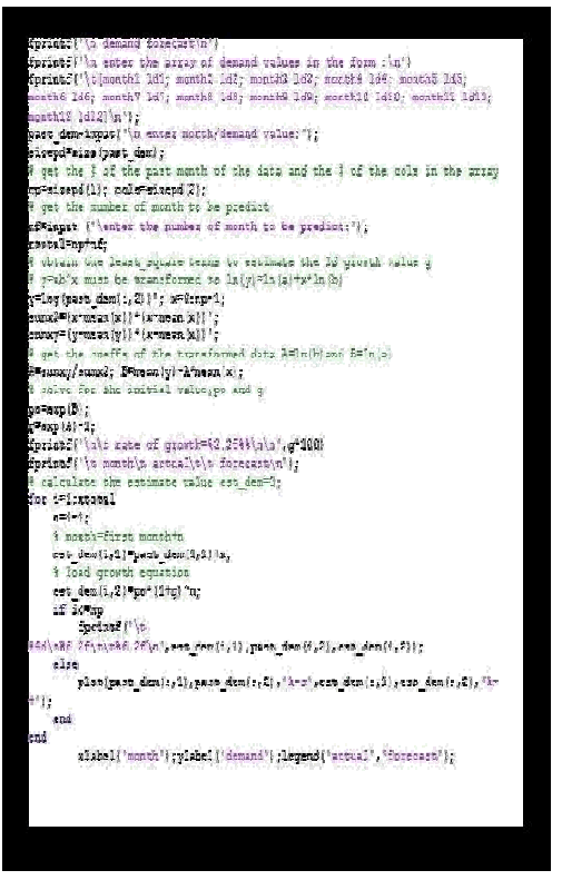
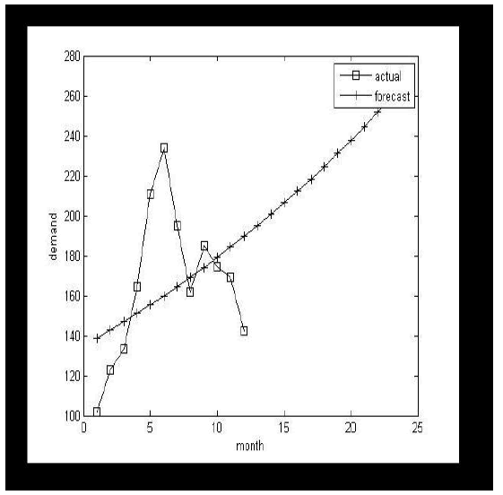
| A simple regression model has been proposed and simulated using MATLAB Simulink. Here a monthly data is taken from TNEB and then put into regression model proposed. We obtain a monthly prediction of load forecasting of STLF. |
 |
 |
Load Forecasted Graph Conclusion: |
| Different techniques have been applied to load forecasting. Six approaches have been reviewed in this paper:(1) Regression Methods(2)Times Series (3)Neural Networks Method (4)Fuzzy Logic Method (5)Knowledge Based Expert System (6)Petri nets system. After surveying all these approaches, we can observe a clear trend toward new, stochastic, and dynamic forecasting techniques. It seems a lot of current research effort is focused on three such methods: fuzzy logic, expert systems and particularly neural networks. There is also a clear move towards hybrid methods, which combine two or more of these techniques. Over the years, the direction of research has shifted, replacing old approaches with newer and more e• |
 |
| efficient ones. Apparently due to their limited success, a number of old approaches seem to be out of favour nowadays. These include such methods as state space and Kalman Filter modelling, on-line load forecasting, and forecasting by pattern recognition. There is also considerably less emphasis on methods such as iterative reweighted least-squares and adaptive load forecasting. |
References |
|