Polish Nuclear Society (PTN), Ul. Dorodna 16, 03-195 Warszawa, Poland
Received date: 10/03/2016 Accepted date: 05/05/2016 Published date: 10/05/2016
Visit for more related articles at Research & Reviews: Journal of Statistics and Mathematical Sciences
The Tadpole Model basing on robust Bayesian regression method is introduced. The paper describes the numerical algorithm for detecting trend changes in the financial quotation or generally - in time-dependent functions. The application of Bayesian fitting algorithm makes the model insensitive to local fluctuations and finally is noise-free. The presented algorithm detects trend changes in Stock Exchange quotations, in the currency exchange rate, etc. The model can work on-line, which means it systematically receives the current value of the analyzed quotation and finds the potential critical and inflection points of the function. The model was tested on the real historical data concerned with several dozens of hourly currency exchange rate and the Warsaw Stock Exchange quotations. About 60% of the model’s trend change detections were correct.
Econophysics, Bayesian, Robust Bayesian regression, Financial quotation, Stock-exchange, Currency.
The data coming from stock-exchange or currency quotation are simple mathematical time functions which can naturally fluctuate. However, in the case of longer time periods, one can notice some regular trends which can vary because of some market signals. Generally, one can enhance such a problem into the analysis of variation of the financial time-dependent functions.
There are many stochastic algorithms which can predict the trend and near future evolution of the financial functions, e.g. [1-6]. However, the stochasticity, usually strictly connected with the frequency probability, can be misleading in the case of the data received on-line. The deterministic approach1 is more appropriate if more precise trend detections can be obtained instead of stochastic predictions.
The presented paper introduces the Tadpole model – the deterministic approach involving the robust Bayesian regression analysis method. The presented algorithm detects trend changes in Stock exchange quotations, in the currency exchange rate etc. The model can work on-line, which means it systematically receives the current value of the analyzed quotation (e.g. a share price), and finds the critical and inflection points of the function. It can potentially affect the decision on buying or selling proper goods. The model can be turned into the main algorithm in a computer program that continuously and automatically conducts financial transactions without human intervention.
The algorithm determines the moment when a local trend potentially changes. It neither establishes the accurate value of a proposed transaction nor conducts it by itself. The Tadpole Model is going to be expanded so that it will perform both functions mentioned before.
The Tadpole Model applies the robust Bayesian regression method, which is very useful in the context of local fluctuations of the data-points. Thus, only the significant changes of trend are detected and fluctuations are omitted. It assists the model in being maximally noise-free.
The presented paper is composed of the following sections:
• The method – where the outline of the robust Bayesian regression analysis is presented,
• The application of the robust Bayesian method to the particular case of detecting trend changes (the Tadpole Model), and
• Results and how the model works in practice.
The Bayes theorem connects the probability of P(Model|Data) with P(Data|Model), which can be used alternatively to the classical probability theory based on the frequency notion. The Bayesian reasoning can be reduced to the simple equation defining the posterior probability [7].
POSTERIOR PROB. = LIKELIHOOD PROB. × PRIOR PROB. (1)
The likelihood function describes some model and its parameters, while the prior function describes degree of belief of the parameter(s).
The robust Bayesian method of regression analysis was comprehensively described in the textbook [7] and applied in [8-13]. The most practical and detailed application was introduced in [9]. Such method of the robust regression can be used for fitting a proper curve to the experimental data points containing outliers (outstanding points creating a noise of data). This method is a good alternative to the least squares regression analysis [14]. The exemplary comparison of both methods is presented in Figure 1 which shows sample data with outlier points. One can clearly see, that outliers makes least squares method very misleading, while Bayesian fit copes well and follows the main trend.

Figure 1: The example of the robust Bayesian (black solid line) and least squares (grey dashed line) fits to some exemplary experimental timedependent data points (t,D) with the three outliers (outstanding points).
The robust Bayesian method defines the posterior probability for each i-th point (eq. 1), which can be presented as the probability density function (PDF) of a normal (Gaussian) distribution
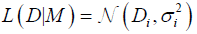 (2)
(2)
as a likelihood function, L, as well as the prior function for its probability σi, proposed by Sivia [7]:
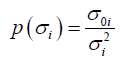 (3)
(3)
Putting the equations (2) and (3) into (1) and using the marginalization procedure, one can present the posterior probability for i-th data point as [7,9,10]:
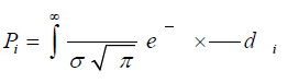 (4)
(4)
where Gaussian residuals equal  for model Mi and time-dependent data Di(ti) (data points (ti,Di), see exemplary Figure 1) with vertical uncertainties σ0i each [9]. The prior function describing σi from eq. (3) assumes that the i-th analyzed probability σi lies between the original one (σ0i) and the infinity. This procedure turns all of the outliers into the insignificant input to the whole posterior probability distribution P for all N points, where, according to the maximum-likelihood estimation method [10], one can use a sum instead of a product:
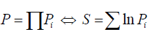 (5)
(5)
where Pi is a result of the integration of eq. (4) for single point i.
After the differentiation of logarithmic probability S with respect to all fitting parameters α={α0,α1,…,αn} of the assumed model M, one can find the final and general form of a Bayesian fitting equation:
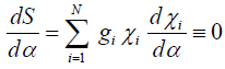 (6)
(6)
where the weights gi of the points are:
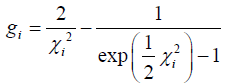 (7)
(7)
The equation (6) can be implemented directly into the computational algorithm to find the best robust Bayesian fit to all N experimental data points (ti,Di) with vertical uncertainties σ0i each [9], like in Figure 1.
The detailed calculations of the presented method, as well as its practical applications, are presented in literature [7-13].
The algorithm presented above can be generalized to the situation, where only some points do outliers need the Bayesian fit, while most of them require only the classical Gaussian (least squares) fitting method. The proper posterior probability function, analogically to eq. (4), which can combine both methods into the single one, can be written as [10-12]:
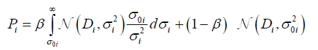 (8)
(8)
where N is a normal (Gaussian) likelihood distribution and β is the probability that data Di is an outlier. It is the reason why the left-hand side of eq. (8) is a Bayesian distribution (same as eq. (4)) and the right-hand the Gaussian one (used finally in the least squares method). This approach is called Mixture of distributions [15] or The good-and-bad data model [7]. One can notice that for β=1 the method (8) became a Bayesian regression, while for β=0 the method became a classical Gaussian one. However, the mixed model works well just for β=0.05 [16], because usually outlier points are the minority among all experimental data [9].
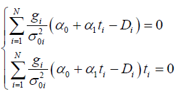
The Bayesian fitting equation (6) is strictly connected with the model (the curve), described as M. Generally, the model M(t) is a time-dependent function which is fitted to the data points (ti,Di) using eq. (6). For fitting parameters α={α0,α1,…,αn} one can use for simplicity the polynomial M(t) = α0 + α1t + … + αntn. In the case of Tadpole Model for i-th point, the M(t) is assumed being linear:
Mi = α0 + α1 (9)
Applying eq. (9) to eq. (6), one can present dedicated simultaneous equations [9]
 (10)
(10)
which can be applied directly to the algorithm for finding estimations of α0 and α1 parameters for linear Mi.
The next feature of the Tadpole Model is the fact, that the time-dependent function (9) fitting to N data points (ti,Di) is a one dimensional multivariable chain [9]:
 (11)
(11)
Each cell from N cells of the chain given by eq. (11) can have their own value of weight, wi:
 (12)
(12)
In practice, the weights wi are introduced as a σ0i=1/wi, where σ0i is the arbitrary vertical uncertainty of i-th point, Di ± σ0i.
The cell for the actual time step (t0) has the highest value of weight (wN) while the rest of the cells have smaller and usually equal weights (w1=w2=…=wN-1). This assumption brings out the analogy between the “head” with high weight and the “tail” with low weight, as in the tadpole’s anatomy. Sometimes one can apply the “neck” (wN-2<wN-1<wN). Figure 2 presents the simple example of a tadpole-like chain (eq. (12)).

Figure 2: The example of a tadpole-like chain for the linear function Mi fitted to some virtual financial data (grey points), where N=7. The thickening of the squaresâÃâ¬Ã⢠sides corresponds to the weight wi. The actual time steps correspond to t0.
In the next time step the chain (12) is moved forward, because the “head” should be always in the beginning (for the actual t0). Generally, for the δt time shift one can calculate the actual values of α0’= α0 + δα0 and α1’= α1 + δα1. The change of α1 is strictly connected both with the trend prediction and the inflection points. The positive value of δα1 is the signal, that trend is increasing. Similarly, the significant change of δα1 between the time steps can be a potential signal that the chain is on the critical or inflection point.
It is difficult to determine the general conditions when the trend change δα1 can be recognized as a significant one. Such conditions depend on many parameters, e.g. the type of data, the potential scattering of the data, the length of the chain (N) etc. It is the reason why the model should be at first calibrated using exemplary historical data. However, this problem can be also solved using the H past time steps (Table 1) – through them one can find the distribution and the standard deviation of H points which can help to assess the type and character of the data scattering and create strict conditions for δα1.
| Symbol | Description |
|---|---|
| Mi | the model (curve) which is fitted to the data using the robust Bayesian regression method; see eq. (9) |
| (ti, Di) | the coordinates of i-th point, where ti is the horizontal coordination (here: the time) and Di is a vertical coordination (the data); see Fig. 1 and 2 |
| wi | the weight of the i-th point (ti,Di); wi is implemented into eq. (4) and (6) as σ0i=1/wi, where σ0i is the arbitrary vertical uncertainty of the i-th point, Di ± σ0i. |
| δt | the time shift which equals ti-ti-1 |
| δα1 | the chain’s slope change after δt |
| N | the number of analyzed points – the length of the tadpole chain, see eq. (12) |
| H | the history – the number of the past points that are kept in the memory |
| B | the time buffer – trend changes are signalized by the time-gap of B to prevent chaotic changes of α1 |
Table 1: The description of symbols used in the presented paper.
All symbols used in the presented paper are described in Table 1.
The presented application of the robust Bayesian regression analysis to financial trend detection has never been fully introduced before, in earlier researches.
The simplified results are presented in Figure 3 where the algorithm was applied to detect trend changes of some simulated exemplary data. However, a few steps delay between the algorithm’s signals and the actual trend changes is the result of scattering prevention, where single outstanding point can be treated as an outlier (Figure 2). This mechanism works better with the actual scattered data (Figure 4).

Figure 3: The result of the application of the algorithm trend detection to simulated exemplary data. Black vertical lines indicate a strong change of ÎôÎñ1 (including the sign change), while grey ones correspond with the soft changes of ÎôÎñ1.

Figure 4: The figure depicts the fragment of GPB/USD ratio as an hourly dependence between 10.05.2009 and 15.05.2009. The moments of trend changes as well as the inflection points found by the algorithm are distinguished as the two types of signals, marked with the black and grey vertical lines, analogically to Fig. 3.
Furthermore, the Tadpole Model with Bayesian regression was also put in an application for the several actual dozens of hourly currency exchange rate (EUR/USD, GBP/USD) and Warsaw Stock Exchange (WIG20) quotations. All of the data were used as an input to the computational algorithm with additional calibration conditions, such as the length of the chain (N=7), history of the scattering (H=20) and the time buffer (B=4) (Table 1). The time buffer, B, was introduced to prevent the chaotic changes of α1 due to the values of wN=2 and wN-1=1.25 (for w1=…=wN-2=1). Thus, the subsequent information on the trend change can usually be available no sooner than B steps after the previous one. On the other hand, the model usually cannot detect the changes faster than B quotations.
About 60% of the inflection or critical point detections were accurate (see Figure 4 for exemplary results). About 70% of the trend direction predictions were also correct. However, the results are strictly connected with the type of the data and input parameters (N, H, B, wi). The model works better with the long-time trend prediction, when fluctuations are rarer than B and the variation of scattered data remains the same at all times.
The model was also tested on the actual on-line data (GPB/USD exchange rate), which gave similar results. All presented results have never been published so far.
The presented Tadpole Model introduces the time-dependent one dimensional chain of points (eq. (12)) fitted to the data acquired on-line using the robust Bayesian regression method (eq. (10)). Such a deterministic approach (in the context of analyzing not only the exemplary made up data, but also the actual ones) differs from many other models of this kind which are based on the stochastic prediction approach (Table 2). The input of the Tadpole Model receives the next quotation e.g. the price of a share or a currency. In order to make the first correct decisions the algorithm needs to both analyzing the sequence of at least N+B+H quotations and being previously calibrated.
| Model and reference | Predictive (P), deterministic (D), mixed (P+D) | Suitable data | Calibration needed? | Outliers resistant? | Selling/buying action proposed? | Base for proper results |
|---|---|---|---|---|---|---|
| (Bartolozzi and Thomas 2004) | P+D | All market and financial data | No | Partially | Yes | Depending on data and parameters |
| (Chang and Feigenbaum 2006) | P | Financial crashes frequency | Yes | Yes | No | Depending on calibration (tested for limited set of data only) |
| (Farahpour et al. 2007) | P | Currency rate | Yes | Partially | No | Depending on data and parameters |
| (Fujiwara et al. 2003) | D | Personal income | No | Yes | No | Depending on data |
| (Renner et al. 2001) | P | Currency rate | Yes | Yes | No | Depending on data and parameters |
| Tadpole Bayesian Model | D | All time related data | Yes | Yes | No | Depending on calibration and type of data |
Table 2: The simple comparison test of main characteristics of the selected econophysical models, including the one described in the presented paper.
The algorithm works through fitting a straight line (model Mi) to the points lying on the graph of a function illustrating the quotation value-to-time dependence. Fitted straight line is a weighted one, which assigns the highest weights for the first points (similarly to the head of a tadpole). However, such determinism causes the delay (which equals a few time steps, ≈B) between the real appearance of the trend change and the algorithm’s signalizing it.
Fitting of the straight line depends on the point’s dispersion that is on the impetuosity (“jumps”) of the single quotation. Provided that the dispersion is small, a straight line can be also fitted by the classical minimization of the χ2 function (the least square method). If the quotation fluctuations are significant, the Bayesian data analysis should be automatically applied. However, the presented model assumes that the robust Bayesian fitting method is always being used.
The Bayesian method of the linear regression requires finding the largest probability (as a result of the multiplication of Pi probabilities for all points) of fitting a straight line to N points described by Gaussian distribution (eq. (4) or (8)). The uncertainties of these points are marked with the prior p(σi), that is in fact the probability distribution. Applying the prior to describe the uncertainties of points results finally in a fitted line basing on the main trend omitting slight trend fluctuations. Owing to this method the algorithm focuses on the actual changes and is not distracted by the accidental deflections [9].
The moment the program detects a trend change (i.e. an inflection of a line that is being fitted) it is signalized by an adequate comment or information sent directly to the main program/user. The algorithm can also predict with high accuracy if the next quotations are going to have an increasing or decreasing trend, or if a single trend type is about to speed up.
One can also enhance the Tadpole Model by implementing the higher value of degree of the polynomial Mi (eq. (9)). Thus, the polynomial curve of the tadpole’s “tail” can be wavy which can improve the effectiveness of the presented method.
The application of the robust Bayesian regression analysis makes the Tadpole Model quite different than the others, thus the clear comparison between them is rather difficult. However, the simple comparison table (Table 2) consists several criteria, which can be used to see main differences in approaches and ways of getting proper results. This comparison clearly indicates that the Tadpole Bayesian Model is a quite good alternative to other existing econophysical models.