Research & Reviews: Journal of Engineering and Technology
ISSN: 2319-9873
ISSN: 2319-9873
Ehab Gomaa1,2*, Mohammed Mnzool2, El-Nagy K. A1,2
1 Department of Mining Engineering, Faculty of Petroleum and Mining Engineering, Suez University, Suez, Egypt
2 Department of Civil Engineering, College of Engineering, Taif University, Taif, Saudi Arabia
Received: 11-Jan-2022, Manuscript No. JET-22-55202; Editor assigned: 13-Jan -2022, Pre QC No. JET-22-55202 (PQ); Reviewed: 27-Jan -2022, QC No. JET-22-55202; Accepted: 31-Jan -2022, Manuscript No. JET-22-55202 (A); Published: 07-Feb -2022, DOI: 10.4172/ 2319-9865.11.2.001.
Visit for more related articles at Research & Reviews: Journal of Engineering and Technology
In a single fan mine, the system characteristic curve represents a relation between airflow and pressure drop across the mine. This relation can be easily drawn in a single fan system by assuming different airflow values and calculating the corresponding pressure drop rendering to Atkinson’s law. In multiple-fan mines, the situation is entirely different, and this cannot be done easily for each fan simultaneously. Moreover, each fan has a partial effect on the ventilation system in the mine. Therefore, it will not work with a specific characteristic curve but has a partial performance curve, subsystem characteristic curve, affected by the known fixed resistances in the mine, and the variable resistances represented by the presence of other fans in the mine. However, each fan subsystem characteristic curve can be achieved by applying an alternative mathematical method for plotting subsystem characteristic curves on subsystem quantity-quantity coordinates or equivalently on the quantity-pressure coordinate. Hardy Cross procedure has been incorporated with a switching-parameters technique to trace subsystem characteristic curves. An example using four fans in a complex network is presented here. This example illustrates the nature of the problem and the difficulty of detecting unstable conditions in this type of network.
Fan characteristic; Multiple fans mines; Ventilation mining network
In any mine a ventilation arrangement is poised of a fan or a group of fans and a set of linked mine ducts. According to Atkinson’s law, the mine characteristic curve in a single fan mine at a specified air weight and a given fan speed is a strictly increasing function. However, this single fan style cannot be directly applying to multiple-fan mines since there are more than one pressures and the same for air quantities related with apiece fan in the system [1]. Therefore, each fan in a several-fan mine has it’s a specific mine characteristic curve or a subsystem curve. Many other investigators have studied the effect of fans on each other in multiple-fan mines. Multiple fans result in an abnormality in the nature of the subsystem curve of each fan and thus result in having several operating points in the system rather than a single point.
In multi-fan mines, a mine characteristic curve does not take the usual form in single-fan mines, which only takes the form of strictly increasing function according to Atkinson’s low. This change in the mine characteristic curve is due to the presence of non-stationary elements such as the presence of other fans and their influence on each other. Therefore, some modifications must be made to the concept of mine resistance before applying it in the laws for calculating the resistance of mine corridors to the air passing through them in mines that have more than one fan inside [2] . Then, the conservative theory of a mine characteristic curve of a single-fan system can be straight drawn-out to that of a specific fan inside multiple-fan mines taking in our consideration the new concept of system resistance. In order to apply the concept of the mine characteristics curve in single-fan mines to one of the fans in multi-fan mines, a set of assumptions must be made on this system [3]. Multi-fan mines do not have a single mine characteristics curve, but there is a mine characteristics curve or subsystem characteristic curve for each fan in the system [4]. In order to obtain this subsystem characteristic curve for each fan, the reference fan must be replaced by a default source of pressure or by adding a constant pressure source without eliminating the fan. Therefore, according to the new concept of subsystem characteristic curve, instead of the conventional characteristic curve for a single mine p in the quantity-pressure level, there are subsystem distinguishing curve for each fan F in the structure [5]. Add to that, there is another set of characteristic curves that are not in the p-q plane, but in the q-q plane or the quantities emitted from each fan. Corresponding qk-pk levels. Where; qk and pk are the quantity and pressure spent over the k subsystem respectively and F is the number of fans in the system. The projection of the solution curve Li on the qi-pi plane represents the characteristic curve of the Pi subsystem of a fan (i). Each Lk solution curve of the k subsystem can be defined by the following equations:


Where M is the number of meshes in the system, q is the air quantity, p is the pressure consumed in the subsystem and f means a function in q1, …,qM that is estimated from Atkinson’s law of mine ventilation, ri |qi| qi where ri is the resistance factor of a branch i. These M equations are represented in M+1 unknown (q1, qM and pi). The solution curve Lk for subsystem i is the locus of all points satisfying these equations represented in an imaginary (M+1) dimensional space [6]. This space is multi-dimensional and is problematic or unbearable to picture if the meshes number (M) in the system is bigger than two, so in this assumption the subsystem characteristic curve is represented as follows:
•Pk: the intersection of the solution curve Lk on the qk-pk plane, and
•Ukij: the intersection of the solution curve Lk on the qi-qj plane (i, j=1…M; i j).
The shape of Pk and Ukij is not distinct, and they are not look like the usual well known regular increasing functions as in a single fan system [7].
The system has more than one solution since the number of unknowns is larger than the number of equations. The conventional techniques that applied to solve nonlinear equations cannot be directly applied to this type of equation because it requires a reasonable initial guess for each solution [8]. Even if the initial estimate is near to the solution point, it may converge either to this point or converge to an old solution point. In addition, one does not know how many solution points are there, so a new technique must be created to solve this system of equations and to conclude the subsystem characteristic curve for each fan [9].
The switching parameter algorithm
One of the effective algorithms for finding multiple solutions to a system of non-linear first-order algebraic differential equations is by switching parameter. The independent variable in this method is undefined and can be changed in every attempt to solve from one variable to another. In this research, a good strategy applied to take the independent parameter at every attempt to solve the equations (1-3) to deduce the solution curve that is the one that changes most quickly. By applying this strategy, it is possible to avoid the interference that may occur as a result of re-solving and passing some parts of the solution curve [10].
For example, Figure 1 shows the relation between two variables x and y. On this curve, at points (e) and (f), the independent variable is x not y that is because the absolute value of the change rate in parameter x in this area of the curve is bigger than the absolute value of the change rate in parameter y (|Δx|>|Δy|) is within the small region adjacent to these (e) and (f). Instead, around points (g) and (h), y is the independent variable, since (|Δy|>|Δx|) | in the small region around these points (g) and (h) (Table 1).
| Interval | Search Direction |
|---|---|
| xa ≥ x ≥| xc | x |
| yd ≥ y ≥ yc | y |
| xb ≥ x ≥ xd | x |
| ya ≥ y ≥ yb | y |
Table 1. Two variables x and y.

Figure 1: Exchanging the independent variable between x and y.
Application of hardy cross to the switching parameters algorithm
As explained before in the multi-fan structure the number of unknown is higher than the number of equation (M) by one. Thus, the only way to solve these types of equations is to assume one of the unknowns (the independent parameter) and solve for the rest of the variables [11]. The independent parameter is undefined, it is fluctuated between the variables at each iterating, and it is not fixed along the entire solution curve. The main purpose of modifying the Hardy Cross method by combining it with the switching parameters algorithm is to enable the optimum selection of the independent variable [12]. In each iteration, the factor that changes most rapidly within its local area, whether increase or decrease will be chosen as the independent variable. It will be treated as a fixed quantity branch and fixed intervals will be algebraically added rendering to the track of the solution path for each iteration stage.
At this step, equations (1-3) are ready to apply the Hardy Cross algorithm until they converge to the appropriate solution. This solution signifies a point in the solution path of a fan subsystem. In order to determine all the solution points and draw the subsystem characteristic curve representing one of the fans installed a mine, these two steps are repeated, choosing the independent factor and treating it as a branch with a fixed quantity, and then applying the Hardy Cross algorithm [13].
Multiple-fan equations have three parameters. They are Resistance Rj, Airflow Rates qj, and Pressure pi (Raj are given for all airways in this work and they will be treated as known parameters) while, qj, and pi are unknowns. As mentioned before the number of unknown exceeds the number of equation by 1. This is because there are M unknown qj in each subsystem K adding to them the unknown pk [14].
In a single fan system, according to Atkinson law, the pressure consumed inside the mine is a strictly increasing function and it is typically treated as the dependent parameter and the airflow as the independent parameter. Likewise, in multiple-fan system, the subsystem pressure drop pk is preserved as dependent and the airflow will be the independent. Therefore, a comparison will be made between the airflow parameters to choose the branch with the largest change in its surroundings and impose it as an independent parameter [15].
Fixed-quantity branch in hardy cross with switching parameter algorithm
The main purpose of applying the normal Hardy Cross method to a branch with a fixed-quantity is to determine the value of the change in the amount of pressure resulting from the installation of a regulator, whether it is an increase in the pressure head by installing a regulator or a decrease in it by an auxiliary fan.
In multi-fan system, there is no extra pressure sources (fans or regulators) are allowed to be installed in any iteration tries. That is because, if any change in the values of pressure is happened means a change will be in the network topology, and the end result is having an another network with dissimilar variables. Thus cut set operation will be applied at each iteration try to distribute the pressure change among the airways. The cut set which include the fixed quantity branch under investigation will be treated as a major cut set in which no change in pressure head is allowed inside the fixed quantity branch. Thus cut set operation will re-adjust the pressures across all brunches and maintain the assigned quantity unchanged through the fixed quantity branch. Thus, the fixed-quantity branches in this system can be classified into a fixed-quantity branch in the major cut set which representing the fan branches, and fixed-quantity branches outside the major cut set. The pressure gain from the fan it is used to distribute the pre-assigned quantity, qi through the fixed-quantity branch which lies inside the major cut set.
The equilibrium between the pressure brought after a fan, it, and the pressure spent by a subsystem, pi is representing a point on the solution curve Lk.
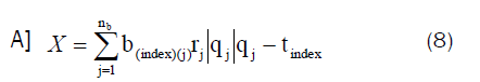
The pressure delivered from the fan is equal the pressure across the fan branch (fixed quantity branch). On the other hand, pressure spent by a subsystem pi is contingent upon resistances of the included branches, and the flow through each of these branches. Therefore, this pressure is not constant at each fixed quantity branch and it is depending upon air quantity through branches. This variance between the pressure gain by fans and the pressure spent through the subsystem is dispersed among the fans within the system by smearing cut set processes on all cutest. Alternatively, if the fixed quantity branch does not belong to the cut set regulator pressure conveyed to the fans in the system by the following ancillary method:
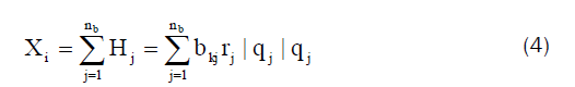
Where Xi is the regulator pressure that is hypothetical to be built in branch i, k is the mesh holding the fixedquantity branch, nb is the number of the branches, Hj is the pressure consumed in a branch j and bkj is an element of the fundamental matrix.
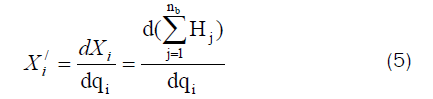
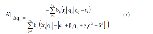
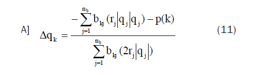
By applying Hardy cross procedure, the improvement rate at every iteration stage is equivalent to Δ(q) i:
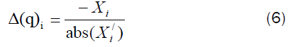
Any change in pressure  in any closed loop will be distributed to all branches except for the branch with a fixed quantity. This correction will be repeated on all closed loops within the network until a satisfactory solution to the network is obtained.
The stages of applying Hardy Cross with the switching parameter algorithm for any network are:
At any subsystem in the network k (j=1, 2… F)
Stage (1): Set standards for the stage size (hq), the primary estimate or the values of air quantity at each airway (Δq), the end limit of iterations (it-no), steps limit (N), lenience rate (max-Δ), and the air quantity inside each branch (q_in).
Stage (2): Assume qj=q_in, for j=1, 2, …, nb.
Stage (3):
• At the primary point in the answer curve, assign the fixed-quantity branch (j) and put qj=hq.
• Then for the rest of the points, find the branch that behave the extreme entire variation (max | [qj (n)-qj (n-1)] |).
Stage (4): If qj(n)>=qj(n-1),let qj(n+1)=qj(n)+hq
Else, let qj(n+1)=qj(n)–hq
Stage (5): Define the initial values as qi=Δ_q.
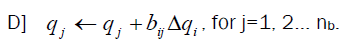
Stage (6): Let qj=qj at the stage (n+1), for
i=1... M.
Stage (7): Estimate, for j=1… nb.
Stage (8): Aimed at the fixed-quantity branch (k), compute p(k)= 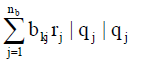
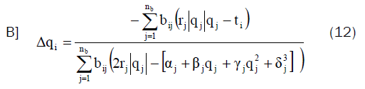
Stage (9): Repeat next estimation for j=1, 2... M: If the fixed-quantity branch (guide) is the identical as branch (k), regulate the pressure delivered from fan (k) to supply p (k) and the apply the next stages;
Where i ≠ k and α,β,γ and δ are the fan coefficients given from the characteristic fan equation.

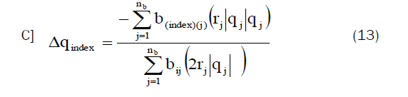
If the fixed-branch (guide) deceits in the same major-cut set with the subsystem fan branch (k) evaluate;
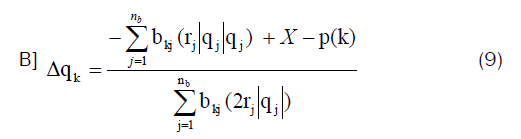
where p(k) is the pressure consumed in subsystem (k) pressure (Pa).
Where i ≠ k ≠ guide.

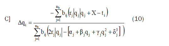
If the fixed branch (guide) doesn't deceits in the same major-cut set branch (k) estimate;
Where i ≠ k ≠ guide
Where guide ≠ i ≠ k
Stage (10): If iterations exceed the limit, go back to stage (5) taking the variable that precedes the second maximum change and treat it as a new a new guide.
Stage (11): The solution is achieved when |Δqi| is fewer than or equivalent to the extreme assigned accepted value, for j=1, 2... M, in stage (9). Then save qj in an array, Qj(stage).
Stage (12): stage=stage+1, repeat the algorithm starting from stage (3).
Stage (13): The mathematical model algorithm will be stop when guide=number of step (k).
Illustrative example to confirm the accuracy of the suggested model
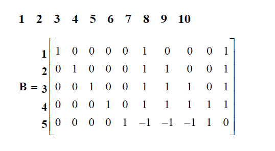
The scheme shown in Figure 2 consists of 10 branches, 6 nodes, and 4 axial flow fans (Table 2). By selecting a tree composed of branches 1, 2, 3, 4, and 5 (as drawn as a bold double line), and then the fundamental mesh matrix concerning the tree can be expressed as:
| Branch # | 1 | 2 | 3 | 4 | 5 | 6 | 7 | 8 | 9 | 10 |
| Resistance, N.s2/m8 | 0.7 | 0.7 | 0.7 | 0.7 | 0.5 | 0.4 | 0.3 | 0.3 | 0.5 | 0.0 |
Table 2. Fundamental mesh matrix concerning the tree.

Figure 2: The network and the resistance for the illustrative case.
There are four fans, therefore, four subsystems. As an example, the system of equations, according to Kirshhoff’s laws and Atkinson’s Equation, associated with the solution curve L is:
r1 |q1| q1+r6 |q6| q6+r10 |q10| q10–P1=0 (14)
r2 |q2| q2+r6 |q6| q6+r7|q7| q7 + r10|q10| q10–t2(q2)=0 (15)
r3 |q3| q3+r6 |q6| q6+r7|q7| q7 + r8|q8| q8+r10 |q10| q10–t3(q3)=0 (16)
r4 |q4| q4+r6 |q6| q6+r7|q7| q7+r8|q8| q8 -r9|q9| q9+r10 |q10| q10–t4(q4)=0 (17)
r5 |q5| q5 -r6 |q6| q6-r7|q7| q7-r8|q8| q8 + r9 |q9| q9=0 (18)
As shown in Table 3, three operating points O1, O2 and O3 have been identified for this ventilation system. Figure 3 shows the intersections between P1, the projection of L1 with the q1-p1 plane, and t1, fan #1 characteristic curve. The operating point’s number in the multiple fan system depends mainly upon the contour of the subsystem characteristic curve and the number of bends it has. For example, the number of operating points in the investigated system could be nine if the subsystem characteristic curve P1 moved up a little bit to intersect with the trough of the fan one characteristic curve. On the other hand, they could intersect only if P1 were to move to down.
| Point | q1, m3/sec | q2, m3/sec | q3, m3/sec | q4, m3/sec |
|---|---|---|---|---|
| O1 | 31.65 | 24.20 | 25.48 | 28.06 |
| O2 | 32.13 | 25.00 | 22.43 | 28.36 |
| O3 | 32.80 | 26.57 | 15.81 | 28.85 |
Table 3. Operating points for the preliminary example.

Figure 3: Subsystem characteristic curve P1.
Similarly, equations associated with L2, L3, and L4 can be driven by using a fundamental matrix (B) and substituting in equations similar to 1 to 3 for P2, P3, and P4, respectively. Figures 4-6 show the first type of subsystem characteristic curves Pi, the projection of the solution curves on in the q-p planes. These figures show the traditional representation of the operating points on the q-p planes. Thus, they can be represented as the intersections between the subsystem characteristic curves for P2, P3, and P4 and the respective fan characteristic curves t2, t3, and t4for fans 2, 3, and 4, respectively. Figures 7-14 show the second type of the subsystem characteristic curves Ukij, the projection of the solution curves k on the qi-qj planes.

Figure 4: Subsystem characteristic curve P2.

Figure 5: Subsystem characteristic curve P3.

Figure 6: Subsystem characteristic curve P4.

Figure 7: Subsystem characteristic curves U112 and U312.

Figure 8: Subsystem characteristic curves U113 and U313.

Figure 9: Subsystem characteristic curves U223 and U323.

Figure 10: Subsystem characteristic curves U212 and U312.

Figure 11: Subsystem characteristic curves U134 and U434.

Figure 12: Subsyste characteristic curves U224 and U324.

Figure 13: Subsystem characteristic curves U123 and U423.

Figure 14: Subsystem characteristic curves U334 and U434.
Consequently, these curves, Ukij, intersect with each other to present a new representation of the operating points as indicated by O1, O2 and O3. For example, Figure 7 shows the intersection of the subsystem characteristic curve U112, the projection of the solution curve of fan #1 on the plane q1-q2, with the subsystem characteristic curve U312, the projection of the solution curve of fan #3 on the q1-q2 plane. As shown in these figures, all the subsystem characteristic curves intersect on three operating points, which show the validity and effectiveness of this model in solving multiple fan networks [16].
A single-fan system can be considered a special case of a multiple-fan system where all of the fans in its subsystems deliver zero pressure at different values of air quantities. A subsystem solution curve may be created in a multiple-fan system that consists of all the solution points of a set of (M) subsystem equations in an (M+1) dimensional space. This solution curve may be projected onto a reference fan’s quantity-pressure plane to represent the subsystem characteristic curve of this fan. Another representation of the subsystem characteristic curve may be drawn by projecting the solution curve onto a quantity-quantity plane. The intersections between the fan characteristic curves and the subsystem characteristic curves represent the operating points of the system. A subsystem characteristic curve delineates a non-zero pressure head at a zero flow rate and it is no longer a strictly cumulative behaves as it would be in a solo-fan scheme. Instead, it may be highly variable and take a zig-zag shape with sharp turning points. This sneaky shape and the number of effective points in the network will be affected by operating parameters such as resistance factors, the topology of the network, fans speeds, number of meshes in the network, and the operating range of the fans in the subsystem.
The application of the Hardy-Cross procedure implemented by switching-parameters technique makes it possible to effectively and efficiently trace an individual subsystem solution curve and identify all the operating points in a complex network by making one primary estimate for the solution.
[Crossref] [Google Scholar] [PubMed]