1Department of Statistics, West Bengal State University, Barasat, India
2International Management Institute, Kolkata, India
Received date: July 06, 2018; Accepted date: July 26, 2018; Published date: July 31, 2018
Visit for more related articles at Research & Reviews: Journal of Statistics and Mathematical Sciences
In this paper we provide a fresh look to the problem of exploration of discrete choice probability, drawing ideas from prospect theory. The deviation of the true choice probability estimates can be attributed to model misspecication and also to the personal choice preference of the individual decision makers. We look at the expressions of choice probability, and explore these in the context of prospect theory and risk aversion of a decision maker. The expression of the distortion of the choice probability with respect to both the above mentioned sources is discussed using the linear in log odds transformation. We then propose that in addition to maximising expected utility of a particular choice, a decision maker should choose a policy that will maximise the estimating power of the true choice probability as a linear ction of the distorted probability. This has been postulated in the form of a theorem, which has been established empirically in the last section of this paper. The current study shows encouraging results for exploiting the nuances of choice probability.
Probability Distortion, Linear in log odds, Multinomial distribution.
The problem of optimal decision making under uncertainty is of paramount importance in every sphere of life and also crucial both to animals and intelligent individuals. Prospective learning advocates that an individual should choose an action that maximizes expected long term gain provided by the environment. To achieve this goal, the individual has to explore its environment, while at the same time exploiting the knowledge it currently has to achieve the goal. In many existing procedure this type of uncertainty is ignored. Practical applications rely on heuristics. In this article we look at the exploration-exploitation trade off from a different perspective- a modified regression theoretic approach. Previous empirical studies have brought to light the fact that while making a decision, decision-makers do not necessarily treat probabilities linearly. In this process the smaller probabilities tend to get under-weighted and the larger probabilities tend to get over-weighted. Kahneman et al. [1] Attributes this phenomena to the use of expected utility by the decision makers and also proposes an alternative method to model decision making. To look at a real life scenario that brings forth this dilemma of the decision makers, let us peruse the following two situations. During the recent recession in 2008, the shares of Indian companies plummeted although the impact of the 2008 recession was somewhat restricted in case of the Indian Market due to a lot of reasons. The first of these is that the Indian financial sector particularly the banks have no direct exposure to tainted assets and hence its off-balance sheet activities are limited. The credit derivatives market was in a nascent stage and there were restrictions on investments by residents in such products issued abroad. India's growth process had been largely Domestic Demand Driven and its reliance on foreign savings had remained around 1.5 percent in recent period. India's comfortable Foreign Exchange Reserves provided confidence in our ability to manage our balance of payments notwithstanding lower export demand and dampened capital flow. Rural demand continued to be robust due to mandated agricultural lending and social safety and Rural Employment Generation programs. India's Merchandise Exports were around 15 per cent of GDP, which was relatively modest. However, since US was one of the major super powers in the world, a recession however mild did have an impact on most of the countries across the globe. As a consequence a lot of the European banks failed and a number of various stock indices declined. This had its effects on India as well since Indian companies have major outsourcing deals from the US, India's exports to the US had also increased substantially over the years. But the impact was over hyped or the probabilities of companies failing and stock prices declining were over-estimated. In such a situation the use of a model which could accommodate distorted probabilities is more befitting.
Again, in another study conducted by Stauffer et al. [2], we can see the role played by a decision maker's choice in distorting choice probability. In this study the same principle is seen to work for Macaque monkeys. While the outcome probabilities are known and acknowledged, it is a tendency of human mind to overweight low probability outcomes and underweight high probability outcomes so as to maximise the reward. Therefore, we investigated economic choices in macaque monkeys for evidence of probability distortion. Parametric modelling of the choices made by the monkeys in the study showed a classic probability weighting functions with inverted-S shape. Therefore, the animals over weighted low probability and underweighted high probability reward. In this study by Stauffer et al. [2] empirically investigated the behaviour of the macaque monkeys and verified that the choices were best explained by a combination of nonlinear value and nonlinear probability distortion. Hence our motivation for revisiting the estimation of discrete choice probabilities, which are otherwise, modelled using the logistic regression model.
In usual regression problem we model the response variable y using an explicit function f(x) such that y = f(x,θ)+є, where є is a random error term and θ is the vector of regression parameters [3]. In case of a simple linear regression, the function f(x,θ) is of the form β0+β1x, which for multiple linear regression, is of the form β0+β1x1+….+βpxp where p is the number of explanatory variables in the model. Through linear regression we model [4] the expected values of the response variable y for given values of X, E(Y|X,θ). Now in cases where we have a binary response, i.e. the response variable only takes two possible values 0 and 1, the above problem is then reduced to one where we model the conditional probability of Y taking the value 1, given X i.e. P[Y=1|X,θ]. The conditional probability models subsume the uncertainty of the model without separating the predictions from the error. The errors are captured by the predictions themselves. In this situation the best model would be the one which would correctly assess the probability of all the possible outcomes and not just attempt to predict the probability of the most likely value. It is this distortion in the probability estimate the has drawn our attention. We have in this paper attempted to find a means of modelling the distortion and tried to explain the source of it.
Our aim in this paper is also to study the diagnostic of fitting a model to estimate choice probability. In section two we aim to derive the distorted probabilities due to model mis-specification and the probability due to personal preference. We would also like to propose a theorem to that end. In section three we prove the proposed theorem empirically.
Theorem 1
Let F(.) be a distribution function corresponding to a random variable then any alternative distribution can be represented
by  , where k > 0 is the distortion parameter that denotes the maximum possible distortion and 0 < p0 < 1, fixed point where F=G.
If k=0 implies degeneracy i.e. G=1
If k=1, F=p0 implies equality of two distribution i.e. G=F
When k > 1(k < 1) implies lower probabilities are overestimated (underestimated) and higher probabilities are underestimated
(overestimated). When there are two equality points except 0 and 1 say at 0 < p1 < p2 < 1 then the alternative distribution can
be represented by 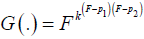 .
.
Let us suppose that we are looking at the preference of one category over another in a decision making problem. This presents us with a discrete choice which can be analysed by techniques such as the logistic regression. The discrete choice model specifies the probability that a person chooses a particular alternative, with the probability expressed as a function of some exploratory variables that are related to the alternatives and the individual making the choice. In this process the probability is expressed as;
Pni=Prob(Individual n chooses alternative i)
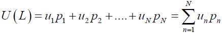
Let us define the probability space (Ω,F,P0), which is all the possible states of the world, F is a sigma algebra of the amount of information available to the experimenter at the time of decision-making and P0 is the probability measure. Then assume that X is a set of random variables on this probability space; X and Y are the two random variables that represent preference. The preference relation is a binary relation which can be represented as X ≥ Y, if and only if U(X) ≥ U(Y) for some real valued function U. Now to model decision problem we usually use a discrete choice models which can be derived from the consumer utility, measure of preference. For any individual the nature is to maximize the expected utility and minimize the risk. The utility function U : L→R has an expected utility calculated from values of utility (u1,u2,…,uN) of the n choices such that there are corresponding probabilities are given by (p1,p2,….,pN). Then the expected utility has the following form;
In case of binary choice model, where the decision maker can only choose between two options the expected utility can be simplified to take the form;
A decision maker is averse to risk if for any cumulative density function F(.), the degenerate preference that yields the amount ∫xdF(x) is with certainty ≥F(.). With a utility function, a decision maker is risk averse if and only if
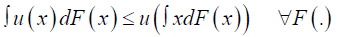
The above condition is called Jensen's inequality and holds for all concave function u(.). Hence risk aversion and concavity of the utility function can be interchangeably used. From previous empirical studies it has been seen that decision makers usually treat probabilities linearly. One way of modelling such distorted probability is through the use of probability weighting functions [1] claim that if there are two logically independent properties to the weighting function, then it is possible to model w with two parameters, one represents curvature (slope) and the other represents elevation (intercept). They proposed the weight function as
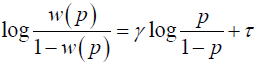
and solving for w(p) we get
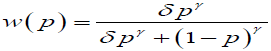 (1)
(1)
where δ= exp(τ). The parameter γ primarily controls the slope and δ controls the intercept. The above functional form (1) is called "linear in log odds". Thus using [5] weight function we can model the distortion in the probabilities.
Similar probability weighting functions have been used in the study carried out by Stauffer et al. [2].
In case of decision under risk different participant in the same experiment can have different distortions and a single participant can exhibit different distortion patterns in different tasks or in different conditions of a single task. Zhang et al. and Qian et al. [6,7] have postulated a two parameter family of transformation to characterize such a distortion in probability. This family is defined implicitly by the following equation
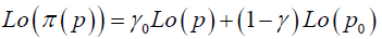 (2)
(2)
where p denotes the true probability and (p) denotes the corresponding distorted probability. Let the distortion in probability due to model fitting be defined as h(p) and the distortion due to the respondents individual preference is given by g(p), then for the true probability p and some fixed point p0 and for some parameters γ and δ we can show that
 (3)
(3)
And with some algebraic manipulation these two equation can give us the true probability as a convex combination of the two distorted probabilities h(p) and g(p) as follows;
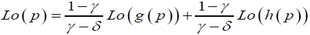 (4)
(4)
 (5)
(5)
where θ=(1- γ)/(γ-δ). The two parameters of the family are quite easily interpreted. In the equation 2, denotes the slope of the linear transformation and the remaining parameter p0 is equivalent to the intercept term. p0 is seldom called the "fixed point", the value of p which is mapped to itself. Here θ determines not only concavity and convexity of probability curve but also through γ and θ we can determine risk and uncertainty associated with a given data point.
Theorem 2
Lo(h(p)) and Lo(g(p)) are both in Euclidean space after the transformation through linear in log odds function. From the expression of the corrected choice probability estimates written as a convex combination of the distorted probabilities, the true choice probability can be best estimated from the distorted probabilities when estimates of both h(p) and g(p) are as close to one another as possible. Fitting a regression model using them as independent and dependent variables respectively, we can estimate the regression coefficient by means of least square as β. With the help of theorem 1 it can be shown that if the regression coefficient is expressed in the exponential form as k(p−p0) , where k is the distortion parameter, then we can get the best possible estimated true probability p.
In a discrete choice problem, we estimate of the choice probabilities under a logistic regression set up. We assume these estimates as the distortion in the probability due to model mis-specification. Again the empirical probability estimates from the observed frequency of each choice can be assumed as the distorted probability due to the personal preference of the decision maker. Under such circumstances, we propose the above theorem and prove it empirically, which is shown in the next section.
For empirical proof theorem 1 postulated in the previous section, we use the data involving variables such as Graduate Record Exam score (GRE) and Grade Point Average (GPA) used to predict the probability of admission into graduate school. The response variable of whether admit/not admit is binary. Using the observed response variable, we can estimate the probability component defined by g(p) in theorem 1.
This component of the true choice probability can be attributed to some extent to the preference of the decision maker. Whereas the probability estimates can depict the distortion in the choice probability due to the model mis-specification. Using the student data we compute the probability g(p), from the model we estimate h(p) using a logistic regression model as follows (Tables 1 and 2);
| g(p) | h(p) | |
|---|---|---|
| 1 | 0.6825 | 0.2374 |
| 2 | 0.3175 | 0.4003 |
| 3 | 0.3175 | 0.5281 |
| 4 | 0.3175 | 0.3153 |
| 5 | 0.6825 | 0.2094 |
| . | . | . |
| . | . | . |
| . | . | . |
| 396 | 0.6825 | 0.4293 |
| 397 | 0.6825 | 0.2483 |
| 398 | 0.6825 | 0.1302 |
| 399 | 0.6825 | 0.4192 |
| 400 | 0.6825 | 0.4013 |
Table 1: Estimates of g(p) and h(p).
| g(p) | h(p) | p | |
|---|---|---|---|
| 1 | 0.6825 | 0.2374 | 0.635 |
| 2 | 0.3175 | 0.4003 | 0.3692 |
| 3 | 0.3175 | 0.5281 | 0.4999 |
| 4 | 0.3175 | 0.3153 | 0.2847 |
| 5 | 0.6825 | 0.2094 | 0.6103 |
| . | . | . | . |
| . | . | . | . |
| . | . | . | . |
| 396 | 0.6825 | 0.4293 | 0.7656 |
| 397 | 0.6825 | 0.2483 | 0.644 |
| 398 | 0.6825 | 0.1302 | 0.5252 |
| 399 | 0.6825 | 0.4192 | 0.7599 |
| 400 | 0.6825 | 0.4013 | 0.7495 |
Table 2: Estimates of g(p) and h(p) along with the corrected estimate of choice probability p.
Risk-aversion is an inherent nature of any decision maker. This aversion dictates their choice and thus in turn it affects their propensity of making any particular choice. Also, when fitting a logistic regression model to obtain the estimate of the choice probabilities there is a possibility of some amount of distortion in the estimate due to a potentially mis-specified model. In this paper we aimed at achieving a corrected estimate if the choice probabilities through some functional form of the two sources of distorted probability. This model thereby shows encouraging results towards maximising the utility of the decision maker.
data<-read.csv(file.choose() , header=T)
model<-glm(admit`gpa+gre , data=data)
summary (model )
hp<-predict (model)
gp=rep (NA, length (hp))
for ( I in 1:length (hp))
{
if (data$admit [i]==1) {
gp[i]<-sum ( data$admit) / length (data$admit )
}
else {
gp [i]<-1-(sum(data$admit) / length ( data$admit ))
}
}
Distort<-function (x,y)
{
ys<-log(-log(y))-log(-log (x))
fbeta=lm (ys`x) $coeff [2]
kappa=exp (fbeta) #exp ( regcoeff (x, lb))
p0=-lm (ys`x) $coeff [1] / fbeta
return ( list ( kappa=as .numeric (kappa) ,p0=as .numeric (p0)))
}
Kappa=distort (gp ,hp ) $kappa
p0=distort (gp ,hp) $p0
p<-hp^ (1 / (( kappa) ^ (gp-p0)))
df=data . frame ( observe=gp, model=hp, corrected=p)
print ( var ( df$observe-df$corrected))
print ( var (df$model-df$corrected))
print ( var (df$observe-df$model))
#Single point distortion
ogive=function (p , kappa=1 , p0=.5) {
p ^ (kappa ^ (p-p0))
}
K1=function (p) ogive (p , kappa = 10)
K_1=function (p) ogive (p , kappa = 0.1)
plot ( ogive , 0 , 1 , xlab=” g(p)”, ylab=”h (p)”, main=” Distortion sing pt .”)
curve ( kl , 0 , 1 , col=2,add=T)
curve ( k_l , 0 , 1 , col=3,add=T)
text ( .5 , .5 ,” p0=0.5”)
text ( .8 , kl (.8) ,” k=10” , col=2)
text ( .2 , k_1 ( .2) ,” k=0.1” , col=3)
#Two point distortion
Ogive2=function ( p , kappa=1 , p1 = .3 , p2=0.7) {
p ^ ( kappa ^ ( (p-p1) * (p-p2)))
}
K21=function (p) ogive2 (p , kappa = 100)
K2_1=function (p) ogive2 (p , kappa = 0.01)
plot ( ogive2 , 0 , 1 , xlab=”g(p)”, ylab=”h (p)” , main=”Distortion two pt .”)
curve ( k21 , 0 , 1 , col=2, add=T)
curve ( k2_1 , 0 , 1 , col=3, add=T)
text ( .3 , .3 ,” p0=0.3”)
text ( .7 , .7 ,” p0=0.7”)
text ( .8 , k21 (.8) ,” k=100” , col=2)
text ( .2 , k2_1 ( .2) ,” k=0.1” , col=3)