P.O. Adebayo* and G.M. Oyeyemi
Department of Statistics, University of Ilorin, Ilorin, Nigeria
Received Date: 12/11/2018; Accepted Date: 23/11/2018; Published Date: 28/11/2018
Visit for more related articles at Research & Reviews: Journal of Statistics and Mathematical Sciences
This work focus on developing an alternative procedure to the multivariate Behrens-Fisher problem by using an approximate degree of freedom test which was adopted from Satterthwaite univariate procedure. The proposed procedure was compared via R package simulation and real-life data used by Tim (1975) with six (6) existing procedures namely: Johanson, Yao, Krishnamoorthy, Hotelling T square, Nel and Van der Merwe and Yanagihara. And it was discovered that proposed procedure performed better in term of power of the test than all existing procedures considered in all the scenarios that are at different: (i) random variables (p), (ii) variancecovariance matrix, (iii) sample size and (iv) significant level (α). And compete favorably well in term of type I error rate with Johanson, Yao, Krishnamoorthy, Nel, and Van der Merwe.
Variance co-variance matrix, linear combination, Type I error rate, power the test, Heteroscedasticity, R statistical package
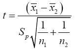
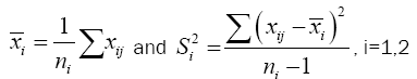
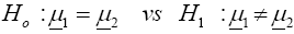
Suppose we have a random sample of size n1, x11, x12, x13, ……x1n1 for N(μ1,σ12) and a second random sample of size n2, x21, x22, x23, . . . x2n2 for N(μ2,σ22 ). It is desired to test H0: u1= u2 against H1: u1≠u2. If σ1 and σ2 are both known a normal test is used. If σ1=σ2 but both are unknown a t-test is commonly used with the test statistics.
Where 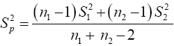
A t-test is a type of statistical test that is used to compare the means of two groups, such as men vs. women, athletes vs. non-athletes, young vs. elderly, or you may want to compare means measured on a single group under two different experimental conditions or at two different times. T-tests are a type of parametric method; they can be used when the samples satisfy the conditions of normality, equal variance, and independence. T-tests can be divided into two types. There is the independent t-test, which can be used when the two groups under comparison are independent of each other, and the paired t-test, which can be used when the two groups under comparison are dependent on each other. If σ1≠σ2 and both are unknown then we are confronted with the Behrens-Fisher problem. There is no universally accepted testing procedure for this problem although arrays of tests have been developed and will be discussed in the Review of Literature. Behrens [1] proposed the statistics.
In the literature, there is a modified test statistic (t-test) when the assumption of equal variances is violated has been known as the Behrens-Fisher problem [1,2]. Early investigations showed that the problem can be overcome by substituting separatevariances tests, such as the ones introduced by Welch [3,4], and Satterthwaite [5], for the Student t-test. These modified significance tests, unlike the usual two-sample Student t-test, do not pool variances in the computation of an error term. Moreover, they alter the degrees of freedom by a function that depends on sample data. It has been found that these procedures in many cases restore Type I error probabilities to the nominal significance level and also counteract increase or decrease of Type II error [6-9].
Student’s t-test is univariate and analog to Hotelling T square which is the multivariate version of T-test and this Hotelling’s T2 has three basic assumptions that are fundamental to the statistical theory: independent, multivariate normality and equality of variance-covariance matrices. A statistical test procedure is said to be robust or insensitive if departures from these assumptions do not greatly affect the significance level or power of the test.
To use Hotelling’s T2 one must assume that the two samples are independent and that their variance-covariance matrices are equal (Σ1=Σ2=Σ). When variance-covariance matrices are not homogeneous and unknown, the test statistic will not be distributed as a T2. This predicament is known as the multivariate Behrens-Fisher problem.
The Behrens-Fisher Problem addresses interval estimation and hypothesis testing concerning the differences between the means of two normally distributed populations when the variances of the two populations are not equal. While Multivariate Behrens- Fisher problem deal with testing the equality of two normal mean vectors under heteroscedasticity of dispersion matrices. These are the some of the existing Multivariate Behrens-Fisher problem: Yao [10], Johansen [11], Nel et al [12], Kim [13], Krishnamoorthy and Yu [14], Gamage et al [15] Yanagihara and Yuan [16],and Kawasaki and Seo [17] and so on. But with all these procedures there is no one with a hundred percent (100%) satisfactory in term of power of the test and type I error rate. And each of these scholars works on the degree of freedom using a different method which is classified into four (4): Approximate degree of freedom tests, Series expansion-based tests, Simulation-based tests, and Transformation-based tests.
Scheffe [18],Lauer and Han [19], Lee and Gurland [20], Murphy [21], Yao [10], Algina and Tang [22], Kim [13], De la Rey and Nel’s [23], Christensen and Rencher [24] , Oyeyemi and Adebayo [25]. All these authors mentioned and many more have work on the comparison of some of the Multivariate Behrens-Fisher problem procedures.
The purpose of this work is to develop an alternative procedure for multivariate data that will be robust compared to other procedures and the work will begin with an introduction to the statistical notation that will be helpful in understanding the concepts. This is followed by a discussion of procedures that can be used to test the hypothesis of multivariate mean equality when statistical assumptions are and are not satisfied. We will then show how to obtain a test that is robust to the covariance heterogeneity.
Consider two p-variate normal populations  and
and where
where  and
and  are unknown p × 1 vector and Σ1 and Σ2 are unknown p × p positive definite matrices.
Let  and
and
 denote random samples from these two populations, respectively. We are interested
in the testing problem
denote random samples from these two populations, respectively. We are interested
in the testing problem
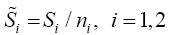
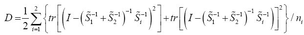
For i=1,2, let
Then  and
and which are sufficient for the mean vectors and dispersion matrices, are independent random variables
having the distributions:
which are sufficient for the mean vectors and dispersion matrices, are independent random variables
having the distributions:
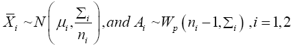
Where Wp(r,Σ)denotes the p -dimensional wishart distribution with df=r and scale matrix Σ.

The following are the existing procedures or solutions to Multivariate Behrens-Fisher problem considered in this study
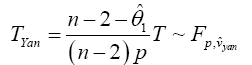
Yao Procedure
Yao [10], invariant test. This is a multivariate extension of the Welch ‘approximate degree of freedom’ solution provided by
Turkey and the test statistic is based on a transformation of Hotelling T2. And is based on 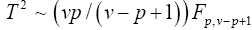 with the
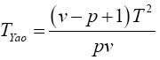
Statistical significance is then assessed by comparing the TYao statistic to its critical value Fα(p,v-p+1), that is, a critical value from the F distribution with p and v–p+1 degrees of freedom (df)
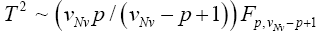
Johansen Procedure
Johansen [11], invariant test, Yanagihara and Yuan [16], Kawasaki and Takashi [17]. They used T2 ~ qFpv where
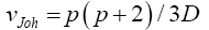
And his proposed test statistic 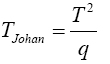
Statistical significance is then assessed by comparing the TJohan statistic to its critical value Fα(p,vJoh), that is, a critical value from the F distribution with p and vJoh degrees of freedom (df).
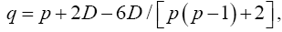
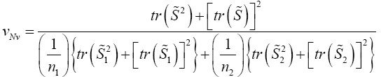
Nel and Van der Merwe (1986) noninvariant solution
Here we use
 except that v is defined by
Krishnamoorthy and Yu (2004)’s, Lin and Wang (2009), Modified Nel/ Van der Merwe Invariant Solution
We use the idea as before, namely,
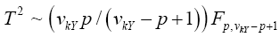 with the d.f.v defined by
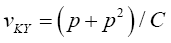

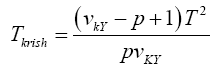
Statistical significance is then assessed by comparing the TKrish statistic to its critical value Fα (p,v_kY-p+1), that is, a critical value from the F distribution with p and v_kY-p+1 degrees of freedom (df)
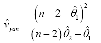
Yanagihara and Yuan Procedure used the Series Expansion Based Test to Developed an Alternative Procedure to Multivariate Behrens-Fisher problem
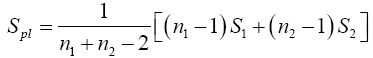
Hotelling’s T2
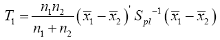
Where
The test statistic can also be converted to an F statistic,
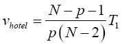
Where N=n1+n2. Statistical significance is then assessed by comparing the vhotel statistic to its critical value Fα (p, N-p-1), that is, a critical value from the F distribution with p and N-p-1 degrees of freedom (df).
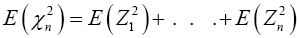
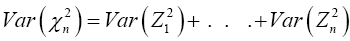
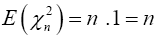
The chi-square distribution is defined with n degrees of freedom by
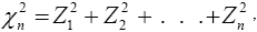 where
where are independent random variables, each with distribution N(0,1).
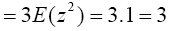
Find the expected value and variance of both sides, then we have
 and
and
And all the instances of Zi have identical distributions, then
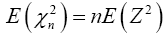 and
and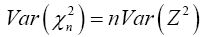
Where Z is the random variable with distribution N(0, 1). Then

Therefore
 (1)
(1)
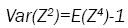
For Var(Z2)

Now
 (2)
(2)
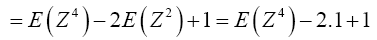
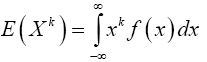
To find E(Z4), we will use the fact that for any continuous random variable X with probability density function f, and any exponent k,
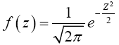
And that the probability density function f of the N(0,1) random variable is given by
Then, 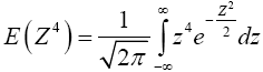
By integration by parts, we have, 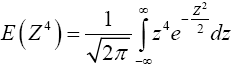
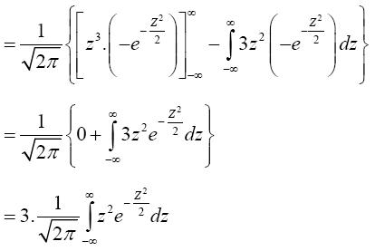
 (3)
(3)
Therefore substitute equation (3) into equation (2) then we have
 (4)
(4)
For two sample t-test, we will limit this work to the version of the test where we do not assume that the two populations have equal variances. Let random sample x1,…,xn1 from a random variable X with distribution N(μ1,σ1) and a random sample y1,….,yn2 from a random variable Y with distribution (μ2,σ2). We have
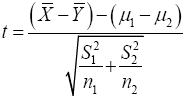 Strictly speaking, this statistic does not follow t-distribution, therefore;
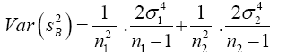
The variance of  is
is and as an estimator for
 we have
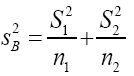
For t to bet–distribution, there would have to be some multiple of  that is chi-square distribution and this is not the case.
However, remember that in the one-sample case,
that is chi-square distribution and this is not the case.
However, remember that in the one-sample case,  had a chi-square distribution with n-1 degrees of freedom. By analogy,
we have
had a chi-square distribution with n-1 degrees of freedom. By analogy,
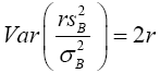
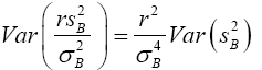
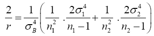
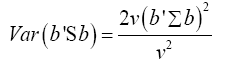
we have  has a chi-square distribution with r degrees of freedom. Satterthwaite found the true distribution of
  and showed
that if r is chosen so that the variance of the chi-square distribution with r degrees of freedom is equal to the true variance of
and showed
that if r is chosen so that the variance of the chi-square distribution with r degrees of freedom is equal to the true variance of  , then, under certain conditions, this chi-square distribution with r degrees of freedom is a good approximation to be the true
distribution of
, then, under certain conditions, this chi-square distribution with r degrees of freedom is a good approximation to be the true
distribution of  so from this point, we are assuming that
 has distribution
 . So from equation (4)
 (5)
(5)
 (6)
(6)
Equating the equation (5) and (6)
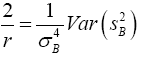 (7)
(7)
Now 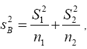 and s1 and s2 are independent so
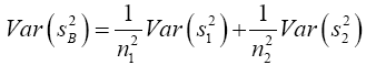 (8)
(8)
We know that  has a chi-square distribution with n1-1 degrees of freedom, from equation (3)
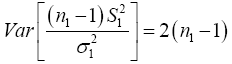
 (9)
(9)
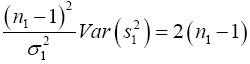
Substitute equation (9) into equation (8)
 (10)
(10)
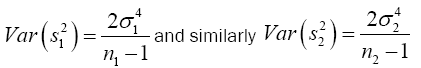
Substitute equation (10) into equation (7)
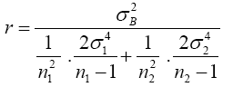 (11)
(11)
In practice, the values of the population variances,  and
and are unknown, and so we replace
 and
and  by their
estimators
by their
estimators  and
and  also
also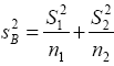 from equation (11)
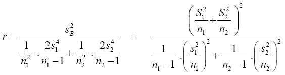
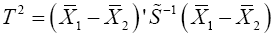
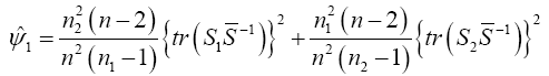
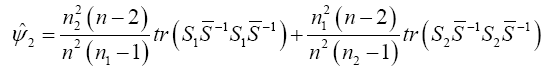
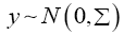
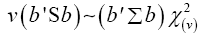
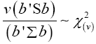
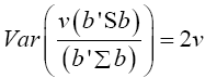
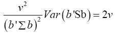
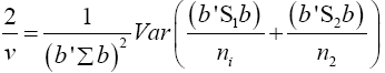
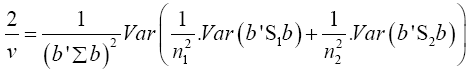
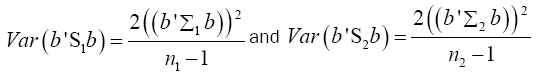
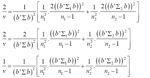
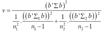
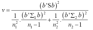
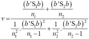
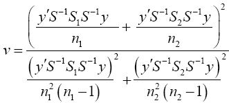
We shall consider the test statistic y'S-1 y and use Univariate Satterthwaite approximation of degrees of freedom method to suggest multivariate generalization based on the T2–distribution. We have
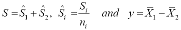
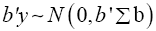
Where b is an arbitrary constant vector
 Multivariate of a version of equation (5)
 (12)
(12)
Multivariate of a version of equation (5) is equation (12)
Note  (14)
(14)
Put equation (14) into equation (13)
 (15)
(15)
Multivariate of a version of equation (9) is
 (16)
(16)
Put equation (16) into equation (15)
 (17)
(17)
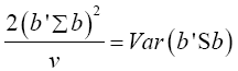
Equation (17) becomes
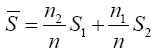
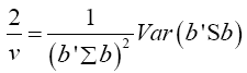
The values of the population variances Σi are unknown, and so we replace Σi and b'Σb by their estimators Si and b'Sb
 (18)
(18)
Put equation (14) into equation (18) to have
 (19)
(19)
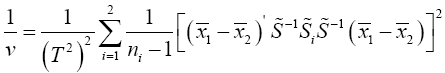
Set b=S-1 y then equation (19) becomes
 (20)
(20)
Equation (20) can be in this form
 (21)
(21)
Let 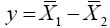 then equation (22) become
 (22)
(22)
 (23)
(23)
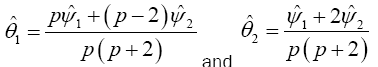
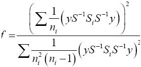
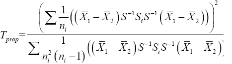
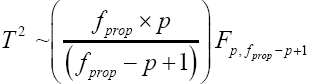
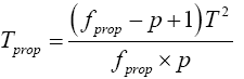
Then equation (23) is the test statistic of the proposed procedure. Statistical significance is then assessed by comparing
the TProp statistic to its critical value 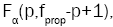 that is, a critical value from the F distribution with p and
  degrees of
freedom (df)
degrees of
freedom (df)
A simulation study using R package was conducted in order to estimate and compare the Type I error rate and power for each of the previously discussed approximate solution [10,11,14], Proposed procedure, Hotelling’s T square, [14,16]. The simulations are carried out when the null hypothesis is true and not true, for Multivariate normal distribution, when there are unequal variancecovariance matrix. Five (5) factors were varied in the simulation: the sample size, the number of variables p, variance covariance matrices, mean vectors, and significant levels. For each of the above combinations, an ni ×p data matrix Xi(i=1 and 2) were replicated 1,000. The comparison criteria; type I error rate and power of the test were therefore obtained and the results were presented in both tabular.
The following are the levels used for each of the three factors.
These levels provide 36-factor combinations the values for sample size are shown in Table 1.
| Multivariate Distribution | P | a | Sample size |
|---|---|---|---|
| Normal | 2, 3, 4 | 0.01 | 20, 10 |
| 2, 3, 4 | 0.025 | 50, 30 | |
| 2, 3, 4 | 0.05 | 100, 60 |
Table 1: Levels used for each of the three factors.
From the Table 2 Nel and Van der Merwe have the highest power of the test when the sample sizes are small (20, 10) but at (50, 30) and (100, 60) the proposed procedure has the highest power than all other procedures.
| P=2 | ÃÆââ¬Å¡Ãâàa=0.01 | |||||||
|---|---|---|---|---|---|---|---|---|
| X1=(20 30) | n1 ≠ n2 | Johan | Yao | Krish | Propo | Hotel | Nel | Yana |
| 20, 10 | 0.3852 | 0.3872 | 0.3872 | 0.3861 | 0.2146 | 0.3915 | 0.2487 | |
| X2=(10 30) | 50, 30 | 0.8332 | 0.8349 | 0.8346 | 0.8374 | 0.6672 | 0.8348 | 0.7691 |
| 100, 60 | 0.991 | 0.9911 | 0.9911 | 0.9912 | 0.9497 | 0.9911 | 0.9865 | |
ÃÆââ¬Å¡Ãâà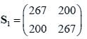 |
ÃÆââ¬Å¡Ãâàa=0.025 | |||||||
| n1 ≠ n2 | Johan | Yao | Krish | Propo | Hotel | Nel | Yana | |
| 20, 10 | 0.5037 | 0.5043 | 0.5045 | 0.5037 | 0.3158 | 0.508 | 0.3787 | |
| 50, 30 | 0.8903 | 0.8911 | 0.8909 | 0.8926 | 0.7609 | 0.891 | 0.8528 | |
 |
100, 60 | 0.9959 | 0.9959 | 0.9959 | 0.996 | 0.973 | 0.9959 | 0.9941 |
| ÃÆââ¬Å¡Ãâàa=0.05 | ||||||||
| n1 ≠ n2 | Johan | Yao | Krish | Propo | Hotel | Nel | Yana | |
 |
20, 10 | 0.6106 | 0.6105 | 0.6104 | 0.6099 | 0.4201 | 0.6133 | 0.5092 |
| 50, 30 | 0.9319 | 0.932 | 0.9319 | 0.9329 | 0.8348 | 0.932 | 0.911 | |
| 100, 60 | 0.9982 | 0.9982 | 0.9982 | 0.9983 | 0.9855 | 0.9982 | 0.9975 | |
Table 2: Power of the test.
From Table 3, when the sample size is (20,10) the proposed procedure is on nominal level exactly while Hoteling T square and Yanagihara [16] are below the nominal level, but at (50,30) and (100,60) all the procedures are below the nominal level, at significant level 0.01. At α=0.025, all the procedures are inflated at (50,30) and deflated at (20,10) and (100,60).
| P=2 | ÃÆââ¬Å¡Ãâàa=0.01 | |||||||
|---|---|---|---|---|---|---|---|---|
| X1=(20 30) | n1 ≠ n2 | Johan | Yao | Krish | Propo | Hotel | Nel | Yana |
| 20, 10 | 0.011 | 0.011 | 0.011 | 0.01 | 0.002 | 0.011 | 0.002 | |
| X2=(20 30) | 50, 30 | 0.007 | 0.007 | 0.007 | 0.007 | 0.001 | 0.006 | 0.004 |
| 100, 60 | 0.008 | 0.008 | 0.008 | 0.008 | 0 | 0.008 | 0.008 | |
| ÃÆââ¬Å¡Ãâà|
ÃÆââ¬Å¡Ãâàa=0.025 | |||||||
| n1 ≠ n2 | Johan | Yao | Krish | Propo | Hotel | Nel | Yana | |
| 20, 10 | 0.017 | 0.017 | 0.017 | 0.018 | 0.003 | 0.018 | 0.005 | |
| 50, 30 | 0.026 | 0.027 | 0.026 | 0.027 | 0.008 | 0.026 | 0.015 | |
|
100, 60 | 0.015 | 0.015 | 0.015 | 0.015 | 0.002 | 0.015 | 0.009 |
| ÃÆââ¬Å¡Ãâàa=0.05 | ||||||||
| n1 ≠ n2 | Johan | Yao | Krish | Propo | Hotel | Nel | Yana | |
|
20, 10 | 0.048 | 0.049 | 0.049 | 0.048 | 0.006 | 0.049 | 0.023 |
| 50, 30 | 0.045 | 0.044 | 0.045 | 0.046 | 0.011 | 0.045 | 0.035 | |
| 100, 60 | 0.057 | 0.057 | 0.057 | 0.057 | 0.016 | 0.057 | 0.051 | |
Table 3: Type I error rate.
From Table 4, It is obvious that proposed procedure performed better than all other procedures at (50,30) and (100, 60) but Nel and Van der Merwe is better when the sample size is (20,10) in all the scenarios considered.
| P=3 | ÃÆââ¬Å¡Ãâàa=0.01 | |||||||
|---|---|---|---|---|---|---|---|---|
 |
n1 ≠ n2 | Johan | Yao | Krish | Propo | Hotel | Nel | Yana |
| 20, 10 | 0.2029 | 0.2198 | 0.2054 | 0.2147 | 0.1313 | 0.2278 | 0.0895 | |
 |
50, 30 | 0.6107 | 0.6182 | 0.6154 | 0.6217 | 0.4472 | 0.6203 | 0.5187 |
| 100, 60 | 0.9295 | 0.9312 | 0.9307 | 0.9322 | 0.8107 | 0.9315 | 0.9073 | |
ÃÆââ¬Å¡ÃâàÃÆââ¬Å¡Ãâà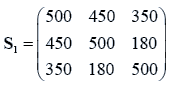 |
ÃÆââ¬Å¡Ãâàa=0.025 | |||||||
| n1 ≠ n2 | Johan | Yao | Krish | Propo | Hotel | Nel | Yana | |
| 20, 10 | 0.2954 | 0.312 | 0.2983 | 0.3062 | 0.206 | 0.3205 | 0.1684 | |
| 50, 30 | 0.7137 | 0.7195 | 0.7173 | 0.7222 | 0.5602 | 0.7209 | 0.6451 | |
 |
100, 60 | 0.9596 | 0.9606 | 0.9603 | 0.9611 | 0.877 | 0.9608 | 0.9478 |
| ÃÆââ¬Å¡Ãâàa=0.05 | ||||||||
| n1 ≠ n2 | Johan | Yao | Krish | Propo | Hotel | Nel | Yana | |
 |
20, 10 | 0.4095 | 0.4255 | 0.4122 | 0.4207 | 0.3002 | 0.4334 | 0.2743 |
| 50, 30 | 0.7952 | 0.7992 | 0.7978 | 0.8012 | 0.6624 | 0.8003 | 0.7475 | |
| 100, 60 | 0.9754 | 0.976 | 0.9758 | 0.9763 | 0.9199 | 0.9761 | 0.9692 | |
Table 4: Power of the test.
Table 5, the type I error rate of all procedures considered are fluctuating, either inflated or deflated. At significant level 0.01, 0.02, 0.05 their inflation in type I error rate, when sample sizes are (50,30) and (100,60), but at (20, 10) all most all the procedures are deflated.
| P=3 | ÃÆââ¬Å¡Ãâàa=0.01 | |||||||
|---|---|---|---|---|---|---|---|---|
 |
Johan | Yao | Krish | Propo | Hotel | Nel | Yana | |
| 20, 10 | 0.007 | 0.008 | 0.008 | 0.006 | 0.014 | 0.013 | 0 | |
 |
50, 30 | 0.011 | 0.01 | 0.011 | 0.09 | 0.013 | 0.011 | 0.006 |
| 100, 60 | 0.015 | 0.015 | 0.015 | 0.015 | 0.018 | 0.015 | 0.013 | |
ÃÆââ¬Å¡ÃâàÃÆââ¬Å¡Ãâà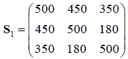 |
ÃÆââ¬Å¡Ãâàa=0.025 | |||||||
| Johan | Yao | Krish | Propo | Hotel | Nel | Yana | ||
| 20, 10 | 0.035 | 0.033 | 0.035 | 0.027 | 0.033 | 0.041 | 0.003 | |
| 50, 30 | 0.025 | 0.027 | 0.026 | 0.024 | 0.032 | 0.028 | 0.011 | |
 |
100, 60 | 0.029 | 0.031 | 0.031 | 0.03 | 0.039 | 0.031 | 0.026 |
| ÃÆââ¬Å¡Ãâàa=0.05 | ||||||||
| Johan | Yao | Krish | Propo | Hotel | Nel | Yana | ||
 |
20, 10 | 0.059 | 0.066 | 0.068 | 0.048 | 0.049 | 0.073 | 0.013 |
| 50, 30 | 0.053 | 0.059 | 0.055 | 0.056 | 0.052 | 0.057 | 0.042 | |
| 100, 60 | 0.061 | 0.061 | 0.062 | 0.061 | 0.056 | 0.063 | 0.051 | |
Table 5: Type I error rate.
Table 6 shows when that sample size is (20,10) Nel and Van der Merwe performed better than other procedures, but when sample size increases to (50,30) proposed procedure is better. And there was a great competition among the procedures at (100,60).
| P=4 | ÃÆââ¬Å¡Ãâàa=0.01 | |||||||
|---|---|---|---|---|---|---|---|---|
 |
Johan | Yao | Krish | Propo | Hotel | Nel | Yana | |
| 20, 10 | 0.343 | 0.3589 | 0.3599 | 0.3508 | 0.1974 | 0.3737 | 0.078 | |
ÃÆââ¬Å¡Ãâà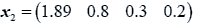 |
50, 30 | 0.86 | 0.8712 | 0.8711 | 0.875 | 0.7027 | 0.8734 | 0.6825 |
| 100, 60 | 0.9968 | 0.9971 | 0.9971 | 0.9973 | 0.9733 | 0.9972 | 0.9902 | |
 |
ÃÆââ¬Å¡Ãâàa=0.025 | |||||||
| Johan | Yao | Krish | Propo | Hotel | Nel | Yana | ||
| 20, 10 | 0.4656 | 0.48 | 0.4817 | 0.4721 | 0.297 | 0.4946 | 0.1604 | |
| 50, 30 | 0.918 | 0.9249 | 0.9247 | 0.9271 | 0.799 | 0.926 | 0.8057 | |
 |
100, 60 | 0.9991 | 0.9992 | 0.9992 | 0.9992 | 0.9888 | 0.9992 | 0.9971 |
| ÃÆââ¬Å¡Ãâàa=0.05 | ||||||||
| Johan | Yao | Krish | Propo | Hotel | Nel | Yana | ||
 |
20, 10 | 0.5662 | 0.5793 | 0.5804 | 0.5731 | 0.3905 | 0.5914 | 0.2585 |
| 50, 30 | 0.9507 | 0.9547 | 0.9547 | 0.9561 | 0.8649 | 0.9555 | 0.886 | |
| 100, 60 | 0.9995 | 0.9996 | 0.9996 | 0.9996 | 0.9938 | 0.9996 | 0.9987 | |
Table 6: Type I error rate
Hotelling T [26] square and yanagihara [16] are below the nominal level in all the scenarios considered, while other procedures fluctuated (Inflated or deflated) round the nominal level as in Table 7.
| P=4 | ÃÆââ¬Å¡Ãâàa=0.01 | |||||||
|---|---|---|---|---|---|---|---|---|
 |
Johan | Yao | Krish | Propo | Hotel | Nel | Yana | |
| 20, 10 | 0.008 | 0.013 | 0.011 | 0.011 | 0.002 | 0.013 | 0 | |
ÃÆââ¬Å¡Ãâà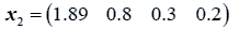 |
50, 30 | 0.011 | 0.012 | 0.012 | 0.012 | 0.001 | 0.012 | 0.002 |
| 100, 60 | 0.007 | 0.007 | 0.007 | 0.007 | 0 | 0.007 | 0.004 | |
 |
ÃÆââ¬Å¡Ãâàa=0.025 | |||||||
| Johan | Yao | Krish | Propo | Hotel | Nel | Yana | ||
| 20, 10 | 0.024 | 0.029 | 0.031 | 0.026 | 0.004 | 0.033 | 0 | |
| 50, 30 | 0.02 | 0.026 | 0.026 | 0.026 | 0.003 | 0.026 | 0.006 | |
 |
100, 60 | 0.021 | 0.022 | 0.022 | 0.022 | 0.002 | 0.022 | 0.01 |
| ÃÆââ¬Å¡Ãâàa=0.05 | ||||||||
| Johan | Yao | Krish | Propo | Hotel | Nel | Yana | ||
 |
20, 10 | 0.05 | 0.055 | 0.055 | 0.051 | 0.009 | 0.06 | 0 |
| 50, 30 | 0.048 | 0.051 | 0.051 | 0.051 | 0.012 | 0.051 | 0.022 | |
| 100, 60 | 0.052 | 0.053 | 0.052 | 0.053 | 0.008 | 0.053 | 0.034 | |
Table 7: Power of the test.
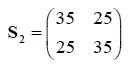
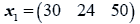
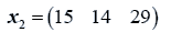
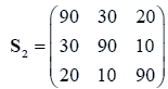
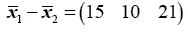
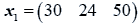
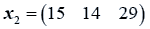
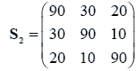
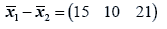
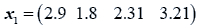
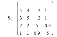
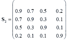
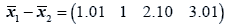
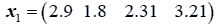
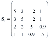
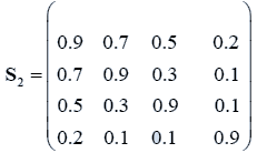
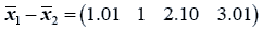
The data used here is an illustrated example used by Timm. The two sample sizes considered are ten and twenty respectively (n1=10 and n2=20) and two random variables (p=2) form each population.
The sample means and their covariances are
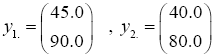
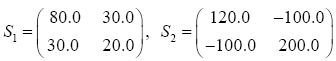
n1=10, n2=20
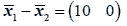
The difference between the means is
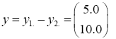
And the test statistic is
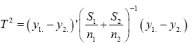
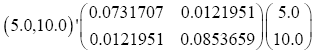
T2=11.58542
From Table 8, the proposed procedure has the highest power followed by Yanagihara [16], Krishnamoorthy [14], Yao [10], Hotelling T square [26], Johansen [11] and Nel and Van der Merwe [14] at all the significant level α considered (α=0.05, 0.025 and 0.01).
| ÃÆââ¬Å¡Ãâàa=0.05 | |||||||
|---|---|---|---|---|---|---|---|
| Johan | Yao | Krish | Propo | Hotel | Nel | Yana | |
| Critical value | 6.978 | 7.2012 | 7.223 | 7.7396 | 6.9567 | 6.9601 | 10.0088 |
| Power | 0.4979 | 0.5109 | 0.5121 | 0.868 | 0.5068 | 0.4969 | 0.6244 |
| ÃÆââ¬Å¡Ãâàa=0.025 | |||||||
| Critical value | 8.852 | 9.1661 | 9.1987 | 9.9867 | 8.7984 | 8.8036 | 13.8708 |
| Power | 0.62 | 0.6334 | 0.6347 | 0.9325 | 0.6273 | 0.618 | 0.7527 |
| ÃÆââ¬Å¡Ãâàa=0.01 | |||||||
| Critical value | 11.4986 | 11.9613 | 12.0129 | 13.2753 | 11.3828 | 11.3908 | 20.3456 |
| Power | 0.7503 | 0.7625 | 0.7638 | 0.9732 | 0.7551 | 0.7456 | 0.868 |
Table 8: The result from the illustrated example.
From the simulation, it is obvious from Tables 1, 3 and 5 that when the sample size is very small (20,10) proposed procedure is not at his best, but when sample size increases to (50,30) and (100,60), the proposed procedure performed better than the all procedures considered. Nel and Van der Merwe [14] performed better when the sample size is very small (20,10) followed by Yao [10], Krishnamoorthy [14] and Proposed procedures in term of power of the test in all the scenarios considered.
In term of Type I error rate, proposed procedure compete favorably well with the other procedures selected for this study. Yao [10], Krishnamoorthy [14], Johansen [11], Nel and Van der Merwe [14] and the proposed procedures are fluctuating (Inflated and Deflated) around the nominal level while Hotelling T [26] square and Yanagihara [16] are below the nominal level.