Forecast and Backtesting of VAR Models in Crude Oil Market

Abstract

The oil price has a very important effect on the world economy. In this paper, using data sets of Europe Brent and West Texas Intermediate (WTI) Cushing crude oil daily prices from Jan. 4, 2000 to Jan. 4, 2016, the VaR forecasting performance of GARCH-type models are analyzed and compared in a short horizon. Based on the Kupiecs POF-test and Christo ffersens interval forecast test, as well as a Back testing VaR Loss Function, the empirical results indicate that, for Europe Brent crude oil, EGARCH (1,1) has the best performance; while for WTI, APARCH (1,1) and GJR-GARCH (1,1) outperform other GARCH models. In fact, these results also give significant guidance on how to choose a better risk management model for the certain commodity of different companies even in the same time period.

Keywords

Risk Metrics, Value-at-risk, GARCH-class models, Forecasting, Backtesting

Introduction

Products of crude oil have been used in many industries, the volatility of crude oil can cause a huge effect on the world economy. From 2010 until mid-2014, the world oil prices had been fairly stable, at around 110 dollars a barrel. But global oil prices fell sharply afterward, and more than halved by winter of 2015. This leads to significant revenue shortfalls in many energy exporting nations, while consumers in many importing countries are benefitted for home heating and the vehicle gas. Large price drops also cause a rise in the volatility/risk of oil market. Therefore, crude oil risk estimation and measurement are crucial for consumers, corporations, governments and internal risk control.

The methods to forecast the oil price and measure its risk are popular topics. The most commonly used measurement for the risk estimation is the Value-at-risk (VaR for short), which measures the maximum loss of a portfolio value over a certain time period at a given level. Identifying proper GARCH-type models with appropriate distributions to evaluate VaR of oil price has become one of most important goals for risk measurement in the crude oil market. Fan et al. [1] estimated VaR of crude oil price using GARCH models, based on the Generalized Error Distribution (GED) and detected extreme risk spillover effect between the two oil markets. Huang et al. [2] employed CAViaR model to forecast oil price risk. Hung et al. [3] investigated the influence of fattailed process on the performance of one-day-ahead VaR estimates about energy commodities using three GARCH models. Wei et al. [4] used several GARCH class models, to capture the volatility of crude oil markets. Marimoutou et al. [5] modeled VaR in the oil market by applying both EVT models to forecast VaR. Aloui [6] computed the VaR using FIGARCH, FIAPARCH and HYGARCH. Youssef et al. [7] evaluated VaR and expected short-fall (ES) using the fitted long-memory GARCH-model, and EVT was used as a potential framework for the separate treatment of tails of distributions.

In order to improve the measure for VaR, an investor needs to estimate the volatility of crude oil price, i.e., risk. Empirical studies have concluded that financial instruments have heteroscedasticity in the variance. To address this observation, the milestones are the ARCH and GARCH, which were introduced by Engle [8] and Bollerslev [9]. Originated from ARCH and GARCH, many new varieties of GARCH models have emerged, which capture the changing volatility over time due to different factors. However there are no definite answers to which of the models from the GARCH family that is the best at forecasting the volatility for all types of financial data. Due to the plethora of different GARCH models available, the models that have been examined need to be restricted to specific data sets. This paper focuses on four of the most influential models, including GARCH (1, 1), EGARCH (1,1), GJR- GARCH (1,1), APARCH (1,1). For detailed constructions, see Bollerslev [9], Nelson [10], Glosten et al. [11] and Ding et al. [12], etc.

The purpose of this paper is to better estimate and forecast the risk of the two crude oil markets - Europe Brent and Cushing, OK WTI. First of all, by Q-Q plot, we conclude that, in both markets, the Student-t distribution fits the log returns significantly (Figure 1). Consequently, we use the Student-t distribution as the preferred conditional distribution for GARCH models in this paper. Secondly, we mainly use Risk Metrics, GARCH (1,1), EGARCH (1,1), GJR-GARCH (1,1) and APARCH (1,1), to study volatility and its corresponding VaR of crude oil, over six years’ time period. Since the performance of a VaR model is determined by how good it predicts future risks. More precisely, for a good VaR model, its estimates of profits and losses should fit the actual profits and losses in some given confident level. However, backtesting with unconditional coverage [13] mainly estimate the number of exceptions, but hardly avoiding the clustering. The conditional coverage by Christoffersen [14] and Haas [15] aims to overcome the clustering by estimating the number of exceptions and the time when they occur, but it cannot catch the long dependence of VaR violations. The duration-based tests of independence (by Christoffersen and Pelletier [16], based on the duration of days between the violations of the VaR, overcomes the clustering and the long dependence of VaR violations. However it relies on estimating of a few parameters. Instead of estimating the violations of the VaR, the method of VaR loss function examines the magnitude of VaR violations. Thus its accuracy relies on the conditional distribution. This paper uses all of these backtesting tools to compare the performances of these models. We conclude that, for Europe Brent, the EGARCH (1,1) outperforms all the other models; while both APARCH and GJR-GARCH specifications are good options for forecasting the VaR for the WTI. It is interesting to note that for both crude oil markets, the worst performing model is the Risk Metrics, which showed no significant results, although it is indeed still popular in many financial institutes.

Figure 1: The upper two plots the spot prices for Europe Brent and WTI; the lower two plots are the associated daily returns.

The rest of this paper is organized as follows. Section 2 introduces the sample data and the statistical characteristics. Section 3 discusses the ve GARCH-type models used in this paper. Section 4 presents the forecasting methodology, the in-sample model t and the out-sample VaR forecasting. Section 5 shows backtesting Value-at-Risk model. Section 6 contains concluding remarks.

Data and Descriptive Statistics

In this paper, we use the daily price data (in US dollars per barrel) of Brent and West Texas Intermediate (WTI) from Jan. 4, 2000 to Jan. 4, 2016. The data is divided into a ten year in-sample period and a six year out-of-sample period. The in-sample period is from Jan. 4, 2000 to Jan.3, 2010 and the rest data are used for out-of-sample forecast and backtesting.

Let p_t be the spot daily price, we consider the log return time series, r_t, defined by

r_t = 100 (log p_t − log p_t−1      (1)

We first examine empirical distribution of the return series by the Q-Q plot. The Q-Q plot of the empirical distribution of the daily returns against the normal distribution is given in Figure 2. It can be observed from the plot that the empirical distributions of both daily returns exhibit heavier tails than the normal distribution. We also perform the Q-Q plot against the student t-distribution, which demonstrates that the empirical distribution of the daily returns fits the t (5)-distribution much better. The unusually high value of the Jarque-Bera statistics in Table 1 shows that the null hypothesis of normality is rejected at the 1% level of significance, also as evidenced by a high excess kurtosis and negative skewness. This is in line with expectations from the ocular inspection of the Q-Q plots in Figure 2, which implied that the empirical distribution of both daily returns exhibit significantly heavier tails than the normal distribution.

Table 1: Descriptive statistics for oil price returns.

Figure 2: Quantile-quantile plot of returns against the normal and the t(5) distribution, respectively.

We also apply two commonly used statistic tests-the Ljung-Box test by Ljung and Box [17] and Lagrange multiplier test [18], which can be applied to check serial correlation of returns and squared returns. In Table 1, the Ljung-Box test result rejects the null hypothesis of no autocorrelation up to the 20th order, and confirms serial autocorrelation in both crude oil returns. ARCH LM test rejects the null hypothesis that there is no auto-correlation for lags 12, at a 1% significance level; and thus confirms that the squared returns are also serially correlated (Figures 1 and 2).

Methodology

Let be all historical information (based on the time series) up to time t. Let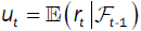 be the conditional return; the volatility. In this paper, to simulate the conditional mean, the AR (1) model is used:

(2)

where , for i = 0; 1.

Next we review various models for estimating the volatility σt. A widely used methodology for measuring market risk is the Risk Metrics, which has become widely used in the financial industry. The main tool is the exponentially weighted moving average (EWMA) method [19], which represents the finite memory of the market. More precisely, the Risk Metrics can be estimated as:

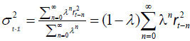(3)

We take λ= 0:94, as most commonly used in the literature.

The Risk Metrics model completely ignores the presence of fat tails in the distribution function, and does not count for the correlations of the return series. In order to over-come these weakness, we use the Generalized Autoregressive Conditional Heteroskedasticity (GARCH) model [9]:

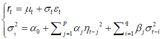
where p > 0; q > 0, and αi,βj are constants, for i = 1,…,p and j = 1,…,q. Here {ε_t} is a white noise with zero mean and unit variance that adapted to The GARCH model is rather popular, as it accounts for persistence of financial time-series data. But it requires that the parameters are not negative, and the models assume that positive and negative shocks have the same impact on volatility. Moreover, it is well known that financial asset volatilities have an asymmetric impact. Typically, the bad news has a greater impact on volatility.

To be able to model this behavior and relax the limitation of parameters, Nelson [10] proposed the Exponential GARCH (EGARCH) model. For p, q > 0, the EGARCH (p,q) model is given by

      (4)

An alternative way of modeling the asymmetric effects of positive and negative asset returns was presented by Glosten, Jagannathan and Runkle [11] resulted in the so called GJR-GARCH (p,q) model, which is given by

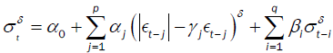    (5)

The asymmetric power ARCH (APARCH) model of Ding et al. [12] is one of the most promising ARCH-type models, and has been studied in many recent applications (see, for example, Giot and Laurent, [20]; Mittnik and Paolella [21]). The APARCH (1,1) model is defined as follows:

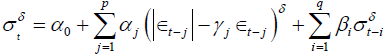
Although it is rather difficult to estimate the order (p; q), some studies have found that the predictive effect of the higher order model is not necessarily better than the low order model, see Hansen PR, Lunde A [22] and Bollerslev T, Chou RY, Kroner KF [23]. Consequently, we choose (p; q) = (1; 1) for various GARCH models in this paper. In addition, we choose the student t (5)-distribution for the error process ε_{_t}. According to our analysis for the empirical distribution of the daily returns, the student t (5)- distribution outperforms the normal distribution.

Model Fitting and Var Estimation

Despite its conceptual simplicity and popularity as an industrial standard in risk management, the estimation of VaR is indeed highly non-trivial. Our goal is to provide a given quantile for the distribution of relative returns of the crude oil. The quantity is defined as the α-quantile of the distribution of the log return, with α chosen as either 95% or 99%:

   (7)

According to the definition and the assumption that ε_t follows the student t (5)-distribution; we know that the α-th quantile of r_t can be calculated as

(8)

where ua denotes the α-th quantile of the student t (5)-distribution. According to the above formula, once we have an estimation for the volatility _t and the expected return _t, the value of VaR can be obtained directly.

We divide the data {r_t, t = 1,…, T} into two subsets. The model parameters are fitted using data in {r_t, t = 1,…, n} (estimation subsample). On the other hand, the forecast of the model is evaluated using data in {r_t, t = n+1,…, T} (forecasting subsample), where n is the initial forecast origin. We are interested in the 1-step ahead forecast, using a so-called recursive scheme. More precisely, one sets m = n to be the initial forecast origin and then fits each of the models using the data r₁, r₂,…, r_m. The 1-step ahead forecasts can now be calculated following the so called fixed scheme. Each model will be fitted to the data until the initial forecast origin from which the forecasts can be computed. Below, we list the forecast formula for our models at forecast origin k, the 1-step ahead forecast:

(1) Risk Metrics:

.

(2) GARCH (1,1):

(3) EGARCH (1,1):

(5) APARCH (1,1):

As previously analyzed, in this paper, we use the standardized t (5)-distribution, so

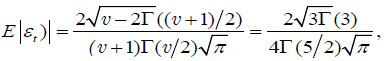     (9)

where v = 5 denotes the number of degrees of freedom and Γ denotes the gamma function. In Table 2 and Table 3, log (L) is the logarithm maximum likelihood function value; AIC is the average Akaike information criterion; Q is the Ljung-Box Q-statistic computed on the standardized residuals. Order of the statistics are reported in brackets. From the p-values of the statistics, the null hypothesis of no autocorrelation is accepted and confirms residual serial no autocorrelation at the 5% levels of significance.

Table 2: Estimation results of different volatility models for Europe Brent crude oil.

Table 3: Estimation results of different volatility models for cushing, OK WTI crude oil.

Backtesting Value-at-Risk Model

In order to help us evaluate the quality of the VaR estimates, the models should be backtested with appropriate methods. Backtesting is to test the accuracy of the model measurement by comparing the actual losses and VaR predictive results.

Unconditional coverage

A popular model to estimate the VaR of financial series is to calculate the number of VaR exceptions, namely days when actual losses exceed VaR predictive results. If the ratio of exceptions is lower than the selected confidence level means that the risk is overestimated. On the other hand, too many exceptions implies the underestimation of risk. Indeed the exact exception suggested by the confidence level is rarely observed. Therefore a statistical analysis is necessary to study whether exceptions are reasonable or not, namely to accept or reject model.

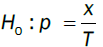
Let x be the number of exceptions and T the total number of observations, hence the failure rate is x=T. In ideal situation, failure rate would be equal to the selected confidence level (Figure 3). If a confidence level is a and let p = 1−α, number of exceptions x obeys a binomial distribution with probability:

Figure 3: One-day-ahead VaR forecasts of Europe Brent crude oil based on the risk metrics and GJR-GARCH models (upper plot), and the GARCH, the EGARCH and APARCH models (lower plot), and the historical volatility.

The accuracy of the VaR model is evaluated through utilizing this binomial distribution. We first use the test suggested by Kupiec [13], which measures whether the number of exceptions is consistent with the confidence level (Figure 4). The null hypothesis for the Kupiec's test is

Figure 4. One-day-ahead VaR forecasts of Cushing, OK WTI crude oil based on the risk metrics and GJR-GARCH models (upper plot), and the GARCH, the EGARCH and APARCH models (lower plot), and the historical volatility.

(11)

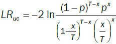
The Kupiec's test statistic is a likelihood-ratio:

(12)

Under the null hypothesis, LR_uc asymptotically follows c2 distributions with one degree of freedom. If the value of LR_uc is greater than the critical value of 3.84, the null hypothesis will be rejected.

Kupiec's test of unconditional coverage is a well-known example of VaR backtest. However, although this test provides a useful benchmark for assessing the accuracy of a given VaR model, this test is hampered by two shortcomings. The first is that this test exhibits low power in sample sizes consistent with the current regulatory framework, i.e., one year. The second shortcoming is that it focuses exclusively on the unconditional coverage property of an adequate VaR measure.

Conditional coverage

Theoretically, we not only focus on the number of exceptions, but also would expect VaR violations to be independent over time. VaR users want to detect clustering of exceptions, because rapid continuous losses than individual exceptions are more likely to lead to catas-trophic events. The most well-known test of conditional coverage has been proposed by Christoffersen [14].

The Christoffersens interval forecast test first de ne an indicator variable:

then define n_ij, I, j = 0, 1, as the number of days when condition j occurred, on the premise of condition I occurred on the previous day. In addition, define π_i as the probability:

(13)

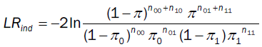
Under the null hypothesis: 0 = 1, the test is conducted as a likelihood-ratio (LR) test with the statistic:

(14)

By combining LR_uc and LR_ind, a joint test is obtained, i.e., conditional coverage:

LR_cc = LR_uc + LR_ind      (15)

LR_cc asymptotically obeys c2 distributions with two degree of freedom.

Duration-based tests of independence

The above tests are efficient at catching whether the probability of an exception on any day depends on the outcome of the previous day. However we are interested in developing tests which have power against more general forms of dependence but which still rely on estimating only a few parameters.

The duration of time between VaR violations (no-hits) should ideally be independent and not clustering. Under the null hypothesis of a correct VaR model, the duration of time between VaR violations should have no memory. Because the only memoryless continuous distribution is the exponential distribution, any distribution which embeds the exponential as a restricted case can be tested. The test can be conducted as a likelihood-ratio (LR) test to see whether the restriction holds. Christoffersen and Pelletier [16] use the Weibull distribution which presents the case of the exponential tail distribution.

Loss function based backtests

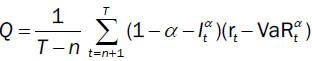
For given α, the loss function Q for the was firstly defined by Gonzalez-Rivera, Lee and Mishra [24]. More precisely,

(16)

where . This is an asymmetric loss function that penalizes more heavily with weight the observations for which . Smaller Q indicates a better goodness of t.

At 95% confidence levels, results of the back tests are shown in Table 4 for Europe Brent crude oil. The unconditional coverage test critical value is 3.841459; and the conditional coverage test critical value is 5.991465. According to the results, Risk Metrics performs the worst, since for both tests, the critical values exceeded with a rather large margin. All GARCH-class models pass both LR_uc and LR_cc tests, with EGARCH model having the best performance. Based on the VaR-based loss function Q, the EGARCH model clearly dominates all the other models [25].

Table 4: Back testing value-at-risk model for Europe Brent crude oil.

For the WTI crude oil, test results are shown in Table 5 with 95% confidence. Again, Risk Metrics performs the worst. All GARCH-class models passed the LR_uc test, while only GJR-GARCH and APARCH passed LR_cc test. Our study shows that GJR-GARCH model has the best performance for the WTI data, with a minimum value for the LR_uc and the LR_cc. According to the VaR-based loss functions Q, the APARCH model outperforms. It is interesting to note that for both crude oil markets, the worst performer is the Risk Metrics method, which is indeed very popular in financial institute as it was first proposed by the JP Morgan Risk Metrics Group [19].

Table 5. Back testing value-at-risk model for cushing, OK WTI crude oil.

Conclusion

In this paper we apply four different GARCH-VaR models with student-t distribution to forecast the conditional variance and its corresponding VaR. The Backtesting indicates that for Europe Brent crude oil, EGARCH (1, 1) model with student-t distribution has the smallest VaR loss, so it will forecast the future VaR better than other models. While for OK WTI crude oil, GJR-GARCH (1,1) and APARCH model under student-t distribution outperform other models. Furthermore, some of results are very useful for companies to choose an appropriate risk management model, which are summarized as the following:

(1) Compared to GARCH model, EGARCH, GJR-GARCH and APARCH are more sensitive for catch asymmetric information.

(2) These results indicate that even for the same commodity (oil), even though we take data sets in same time interval, the commodity of different country/companies may have a different appropriate model to predict the future VaR.

(3) We can amplify the conclusion of (2): even for the same commodity of same country/companies, in different time periods, an appropriate model to predict its future VaR may vary too. These conclusions give significant guidance for companies to choose a better risk management model based on the statistical properties of the time series, in a certain time period.

The above analysis indicates that, whenever we want to forecast the value at risk for a commodity of a company in a short horizon, it is always better to compare all of models to choose an appropriate one, as there is hardly any model that fits a commodity forever.

Acknowledgements

HK Zhang is supported in part by NSF grant DMS-1151762, as well as the Simons Fellow-ship.

References

1. Ying Fanet al. Estimatingvalue at risk of crude oil price and its spillover effect using the GED-GARCH approach, Energ Econ. 2008;30:3156-3171.
2. Dashan Huanget al.CAViaR-based forecast for oil price risk. Energ Econ. 2009;31:511-518
3. Jui-Cheng Hunget al. Estimation of value-at-risk for energy commodities via fat-tailed GARCH models, Energ Econ. 2008;30:1173-1191
4. Yu Weiet al. Fore-casting crude oil market volatility: Further evidence using GARCH-class models, Energ Econ. 2010;32:1477-1484
5. VelayoudoumMarimoutouet al. Extreme value theory and value at risk: Applications to oil market.Energ Econ. 2009;31:519-530
6. ChakerAloui and Samir Mabrouk. Value-at-risk estimations of energy commodities via long-memory, asymmetry and fat-tailed GARCH models. Energy Policy. 2010;38:2326-2339
7. Manel Youssef et al. Value-at-risk estimation of energy commodities: A long-memory GARCH?EVT approach. Energ Econ. 2015;51:99-110
8. Engle RF. Autoregressive conditional heteroskedasticity with estimates of the variance of United Kingdom in ation. Econometrica. 1982;50:987-1007
9. Bollerslev T.Generalized autoregressive conditional heteroskedasticity. J Economet, 1986;31:307-327.
10. Nelson DB. Conditional heteroskedasticity in asset returns: A new approach. Econometrica.1991; 59:347-370.
11. Glosten LRet al. On the relation between the expected value and the volatility of the nominal excess return on stocks.J Finance. 1993;48:1779-1801.
12. Ding Z et al. A long memory property of stock market returns and a new model. J Empirical Finance. 1993:1;83-106.
13. Kupiec P. Techniques for verifying the accuracy of risk management models.J Derivatives 1995;3:73-84.
14. Christofferssen P. Evaluating interval forecasts.Int Econ Rev. 1998;39:841-862.
15. Haas M. New methods in backtesting, Financial Engineering, Research Center, Caesar, Bonn. 2001.
16. Christoffersen P and Pelletier D. value-at-risk: A duration-based approach. JFinancEconometr. 2004;21:84-108.
17. LjungGM and Box GEP. On a measure of a lack of fit in time series models. Biometrika. 1978;65: 297-303.
18. Robert FE. A general approach to lagrange multiplier model diagnostics. J Econometrics. 1982;201:83-104.
19. RiskMetrics Group. Riskmetrics-Technical document, New York: JP. Morgan/Reuters, 1996.
20. Giot P and Laurent S. Market risk in commodity markets: aVaR approach. Energ Econ. 2003;25:435-457.
21. Mittnik Set al. Conditional density and value-at-risk prediction of Asian currency exchange rates. J Forecast. 2000;19:313-333.
22. Hansen PR and Lunde A. A forecast comparison of volatility models: Does anything beat a GARCH 1.1. J ApplEconometr. 2005;20:873-889.
23. Bollerslev T et al. ARCH modeling in finance: Areview of theory and empirical evidence. J ApplEconometr. 1992;52:5-59.
24. Gonzalez-Rivera G, et al. Forecasting volatility: A reality check based on option pricing, utility function, value-at-risk, and predictive likelihood. Int J Forecast. 2004;204:629-645.
25. Campbell S. A review of backtesting and backtesting procedure, Finance and Economics Discussion Series, Divisions of Research and Statistics and Monetary affairs, Federal Reserve Board, Washington DC. 2005.