Keywords
|
| demosaicking, bayer filter, CFA, interpolation, zippering, correlation, PSNR |
INTRODUCTION
|
| Digital images are formed by interpolating the CFA. Here we use the Bayer CFA (as shown in Fig.1).The Bayer CFA contains a mosaic of pixels where each pixel has any one spectral measurement of the chrominance(red and blue) and luminance(green). Bayer CFA has 50% green values and 25%-25% of the red and blue values arranged in a specified lattice pattern[1]. For any color image a pixel must have all the RGB components. Using the Bayer CFA results in only one component(out of R,G,B) at a pixel. To reconstruct a full color image the missing color components have to be estimated. Demosaicking is the method of reconstructing a color image by calculating the missing pixel values[2]. Calculation of missing values can be done with the help of interpolation and as well as interchannel correlation[3].Interpolation techniques can be nearest-neighbour, bilinear and cubic spline interpolation. Interpolation using color correlation gives better performance as there is high correlation in R, G and B components[4][5]. In Bayer pattern, output image suffers from alternating colors, often referred to as zippering, artifacts[2]. They are the unwanted features(as shown in Fig.3) which do not appear in original image(Fig.2). |
LITERATURE SURVEY
|
| Demosaicking methods can be grouped into two different groups-(i) applying interpolation techniques to each color channel separately and (ii)by using the inter-channel correlation. Interpolation techniques in first group includes nearest neighbour, bilinear and cubic splines interpolation whereas few approaches in latter are edge directed interpolation and smooth hue transition. Interchannel correlation results in better images[3].The algorithm proposed by Gunturk[3]used a combined approach of alternating projections in which bilinear interpolation was used for red and blue channels and for green channel edge-directed interpolation. Using an iterative scheme edge directed interpolation and smooth hue transitions were combined and implemented[5]. It is named as the Kimmel algorithm. The basic steps involved in this algorithm are- (i) interpolate green color,(ii)interpolate the red and blue color using the green and (iii)correction stage[6]. This algorithm almost eliminated the zipper effect artifact. Another algorithm based on optimal recovery and Kimmel algorithm results in a better image due to highly complicated interpolation of the green channel. This algorithm was named as AQua-2 algorithm. If the color direction vector coincides with the gray color axis, in that case Alternating Projection method works well. All the advantages of these methods were combined altogether and when implemented produced better results[6]. Table I shows the results on the basis of PSNR measured in dB. |
| Due to high correlation of R, G and B channels interpolation using color correlation was used. Crosscorrelation between the channels were determined and observed that they vary between the range of 0.25 and 0.99 with average values of 0.86 for red/green, 0.92 for green/blue and 0.79 for red/blue[1]. |
| In another method, for interpolation of G channel we can use the information of R and B channels[7]. Based on the model developed by J.E Adams,Jr.[8], two constants were introduced KB and KR . The values of both can be calculated as KB = G - B and KR = G - R. Instead of interpolating values domain-wise the entire calculation is transformed into these new introduced constants. To calculate the value of G at R7, we have to calculate K values for both R and B respectively. To estimate R3 average of R1 and R7 is used and for calculating R6 average of R5 and R7 is used. Finally the values will be |
| K'R3 = G3 - R'3 = G3 - (R1 + R7) / 2 and |
| K'R6 = G6 - R'6 = G6 - (R5 + R7) / 2. |
| The G channel performs 6.34dB improvement over bilinear method and on an average 7.69dB improvement on R,G and B channels[7].Ideal interpolation has not been implemented in practice[1]. |
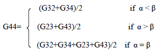
| In Median-based interpolation proposed by Freeman, was a two step distinct process. In the first step linear interpolation was done and the second step was using median filter of the color differences on 3x3 window[9]. For speckle behaviour in images Freeman's algorithm can be used. Gradient based interpolation proposed by Laroche and Prescott uses three steps in the algorithm. In first step the green channel is interpolated and in second and third step comprises of interpolation of the color differences(red-green, blue-green)[10].This algorithm is suitable for images with sharp edges. It is implemented as follows: To calculate G44 we use classifiers, α and β which will determine whether a pixel belongs to a vertical or horizontal edges respectively. The estimates can be calculated as: |
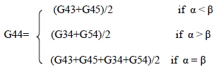 |
| For estimating G33, let α=abs[(R31+R35)/2 - R33] and β=abs[(R13+R53)/2-R33]. |
 |
| Once luminance is determined, chrominance values are interpolated by calculating the difference of the luminance and the red-blue signal. It is calculated by |
| R34 =[ (R33 - G33) + (R35 - G35)] / 2 + G34; |
| R43 =[ (R33 - G33) + (R35 - G35)] / 2 + G43; |
| R44 = [(R33 - G33) + (R35 - G35) + (R53 - G53) + (R55 - G55)] / 4 + G44 |
| Adaptive color plane interpolation suggested by Hamilton and Adams [11] is a modification of gradient based interpolation. The classifiers are defined as - |
| α = abs (-A3 + 2A5 - A7) + abs (G4 - G6) |
| β = abs (-A1 + 2A5 - A9) + abs (G2 - G8) |
| To estimate G5,it can be determined as- |
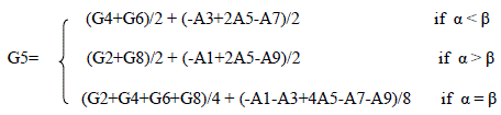 |
BASIC METHODS USED IN DEMOSAICKING
|
| A. Bilinear Method: |
| Color images are used here(jpg format). To perform demosaicking, bilinear interpolation is used. For bilinear interpolation, nearest pixels are taken into consideration. To obtain the separate color channels of each pixel the image is first made to pass through a bayer filter(shown in fig.1). This filter has a specialty of absorbing only one channel value per pixel. They may be arranged in RGBG,GRGB,RGGB patterns, depending upon the value of first pixel, later arranged in a lattice structure. The formula for bilinear interpolation is, to calculate value of R,G and B components at pixel position 13, the corresponding values can be calculated as: |
| R13 = R13 (as red component is already present there) |
| We now need to estimate the values of G and B components- |
| G13 = (G8 + G12 + G14 + G18) / 4; |
| B13 = (B7 + B9 + B17 + B19) / 4 |
| For corner pixel at position 5 the values are calculated using the following formula- |
| R5 = R5; |
| G5 = (G4 + G10) / 2; |
| B5 = B9 |
| B. Edge Sensing Method: |
| It is a type of Adaptive algorithm[12], in which horizontal and vertical classifiers are used to determine whether an edge is present or not. The classifiers are named as ΔH and ΔV. To calculate G13 we will use the following formula- |
| G13H = (G12 + G14) / 2; |
| G13V = (G8 + G18) / 2; |
| G13A = (G8 + G12 + G14 + G18) / 4; |
| ΔH = |G12 - G14|; |
| ΔV = |G8 - G18|; |
| A threshold value T is selected and then comparing the values of ΔH and ΔV, the appropriate value is assigned for the corresponding pixel. It is depicted in the following flowchart (Fig.4) |
| C. Signal Correlation Method: |
| In signal correlation method instead of using horizontal and vertical classifiers, the entire scheme was transformed to KB and KR domains[7]. |
| For G channel interpolation- |
| G'13 = R13 + (KR'8 + KR'12 + KR'14 + KR'18) / 4 |
| KR' = G - R; |
| KB' = G - B; |
| R and B channel interpolation- |
| R'8 = G8 - (KR'7 + KR'9) / 2; |
| B'13 = G'13 - (KB'7 + KB'9 + KB'17 + KB'19) / 4 |
| The images on which these above mentioned algorithms were implemented are shown in figure below(Fig.5). |
SIMULATION RESULTS
|
| To evaluate the algorithms simulations were conducted on test images[13] and to evaluated on the basis of PSNR(Peak Signal to Noise Ratio) measured in dB. Separating the r, g and b channels and measuring the PSNR with the original images calculated and the values have been shown in Table II[7]. |
CONCLUSION
|
| The algorithm evaluation was done on 4 test images[13] channel-wise separately and it was found that Signal Correlation Method gave better results[7] as 6-7dB improvement was noted in the green channel and 4-5dB improvement was observed in red and blue channels separately. The complexity of this method is acceptable. |
Tables at a glance
|
 |
|
| Table 1 |
Table 2 |
|
| |
Figures at a glance
|
 |
 |
 |
 |
 |
| Figure 1 |
Figure 2 |
Figure 3 |
Figure 4 |
Figure 5 |
|
| |
References
|
- Ramanath, R. , Snyder, W. E. , Bilbro, G. L. , and Sander III, W. A. , “Demosaicking methods for Bayer color arrays”, Journal of Electronic Imaging, Vol.11( 3), pp. 306–315,July 2002.
- Hirakawa, K. ,Parks, T.W. , "Adaptive homogeneity-directed demosaicing algorithm", IEEE Transactions on Image Processing, Vol.14(3), pp. 360-369, 2005.
- Gunturk, B. K. ,Altunbasak, Y. , and Mersereau, R. , “Color plane interpolation using alternating projections”, IEEE Transactions on Image Processing, Vol. 11(9), pp.997–1013, Sept. 2002.
- T. Kuno, and H. Sugiura “New Interpolation Method Using Discriminated Color Correlation for Digital Still Cameras”, IEEE Trans. Consumer Electronic, Vol.45(1), pp. 259-267 ,Feb. 1999
- R. Kimmel, “Demosaicing: Image Reconstruction from Color CCD Samples”, IEEE Trans. Image Processing, Vol. 8(9) , pp. 1221-1228, Sep. 1999.
- Lukin, A. ,Kubasov, D. , “High-Quality Algorithm for Bayer Pattern Interpolation”, Programming and Computer Software, Vol. 30(6), pp. 347–358, 2004.
- Pei, S.C. , and Tam, I.K. , “Effective color interpolation in CCD color filter arrays using signal correlation”, IEEE Transactions on Circuits System. Video Technology, Vol 13(6), pp. 503–513, June 2003.
- Adams, Jr. J. E. , “Design of Practical Color Filter Array Interpolation Algorithms for Digital Cameras”, Proceeding of SPIE, Vol. 3028, pp. 117- 125, 1997.
- Freeman, W.T. , "Median filter for reconstructing missing color samples", U. S. Patent No. 4,724,395(1988).
- Laroche, C. A. , and Presscott, M. A. , "Apparatus and method for adaptively interpolating a full Color image utilizing chrominance gradients", U.S.Patent No. 5,373,322 (1994).
- Hamilton, J. F. , an Adams, J. E. , "Adaptive color plane interpolation in single sensor color electronic camera'' ,U.S. Patent No. 5,629,734(1997).
- Adams, Jr J.E. , “Interactions between Color Plane Interpolation and Other Image Processing Functions in Electronic Photography” ,Proceeding of SPIE, Vol. 2416, pp. 144-151, 1995.
- Kodak Lossless True Color Image Suite[EB/OL]. http: //rok.us.graphics/kodak/,1999.
|