Keywords
|
| Feature extraction, feature matching, MFCC, LPC, PLP, ANN, HMM, DTW, Vector Quantization, Gaussian Mixture Model. |
I. INTRODUCTION
|
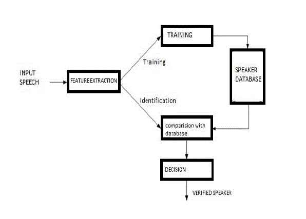
| Human voice conveys information about the language being spoken and the emotion, gender and, generally, the identity of the speaker. Speaker recognition is a process where a person is recognized on the basis of his voice signals [1, 2]. The Objective of speaker recognition is to determine which speaker is present based on the individual’s utterance. This is in contrast with speaker verification, where the objective is to verify the person’s claimed identity based on his or her utterance. Speaker identification and speaker verification fall under the general category of speaker recognition [3, 4]. |
| In speaker identification there are two types, one is text dependent and another is text independent. Speaker identification is divided into two components: feature extraction and feature classification. In speaker identification the speaker can be identified by his voice, where in case of speaker verification the speaker is verified using database. |
| The Pitch is used for speaker identification. Pitch is nothing but fundamental frequency of a particular person. This is one of the important characteristic of human being, which differ from each other. The speech signal is an acoustic sound pressure wave that originates by exiting of air from vocal tract and voluntary movement of anatomical structure. |
| The human speech contains numerous discriminative features that can be used to identify speakers. Speech contains significant energy from zero frequency up to around 5 kHz. The objective of voice recognition is to extract, characterize and recognize the information about speaker identity. |
II. SPEECH RECOGNITION PROCESS
|
| The goal of speech recognition is for a machine to be able to "hear,” understand," and "act upon" spoken information. The earliest speech recognition systems were first attempted in the early 1950s at Bell Laboratories, Davis, Biddulph and Balashek developed an isolated digit Recognition system for a single speaker [5]. The goal of automatic speaker reorganization is to analyze, extract characterize and recognize information about the speaker identity. The speaker reorganization system may be viewed as working in a four stages. |
| 1) Analysis |
| 2) Feature extraction |
| 3) Modeling |
| 4) Testing |
III. FEATURE EXTRACTION
|
| Feature Extraction is the most important part of speech recognition since it plays an important role to separate one speech from other. Because every speech has different individual characteristics embedded in utterances. These characteristics can be extracted from a wide range of feature extraction techniques proposed and successfully exploited for speech recognition task. But extracted feature should meet some criteria while dealing with the speech signal such as: |
| 1) Easy to measure extracted speech features |
| 2) It should not be susceptible to mimicry |
| 3) It should show little fluctuation from one speaking environment to another |
| 4) It should be stable over time |
| 5) It should occur frequently and naturally in speech |
| The most widely used feature extraction techniques are explained below. |
| A. MEL FREQUENCY CEPSTRAL COEFFICIENT (MFCC) |
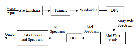
| A block diagram of an MFCC feature extraction is shown (Fig. 2).This coefficient has a great success in speaker recognition application. The MFCC [6] [7] is the most evident example of a feature set that is extensively used in speech recognition. As the frequency bands are positioned logarithmically in MFCC [8], it approximates the human system response more closely than any other system. Technique of computing MFCC is based on the short-term analysis, and thus from each frame a MFCC vector is computed. In order to extract the coefficients the speech sample is taken as the input and hamming window is applied to minimize the discontinuities of a signal. Then DFT will be used to generate the Mel filter bank. MFCC can be computed by using the formula (1). |
| Mel (f) = 2595*log10 (1+f/700) (1) |
| The following figure 2 shows the steps involved in MFCC feature extraction. |
| B. LINEAR PREDICTIVE CODING (LPC) |
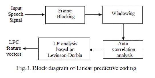
| Linear prediction is a mathematical computational operation which is linear combination of several previous samples. LPC [6] [7] of speech has become the predominant technique for estimating the basic parameters of speech. It provides both an accurate estimate of the speech parameters and it is also an efficient computational model of speech. The basic idea behind LPC is that a speech sample can be approximated as a linear combination of past speech samples. Through minimizing the sum of squared differences (over a finite interval) between the actual speech samples and predicted values, a unique set of parameters or predictor coefficients can be determined. These coefficients form the basis for LPC of speech [9]. The following figure 3 shows the steps involved in LPC feature extraction. |
| C. PERCEPTUAL LINEAR PREDICTION (PLP) |
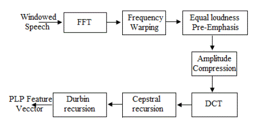
| The Perceptual Linear Prediction (PLP) model developed by Herman sky 1990. The goal of the original PLP model is to describe the psychophysics of human hearing more accurately in the feature extraction process. PLP is similar to LPC analysis, is based on the short-term spectrum of speech. In contrast to pure linear predictive analysis of speech, perceptual linear prediction (PLP) modifies the short-term spectrum of the speech by several psychophysically based transformations. |
IV. FEATURE MATCHING / CLASSIFIER
|
| The speech feature extraction in a categorization problem is about reducing the dimensionality of the input vector while maintaining the discriminating power of the signal. As we know from fundamental formation of speaker identification and verification system, that the number of training and test vector needed for the classification problem grows with the dimension of the given input so we need feature extraction of speech signal. |
| A. ARTIFICIAL NEURAL NETWORK (ANN) |
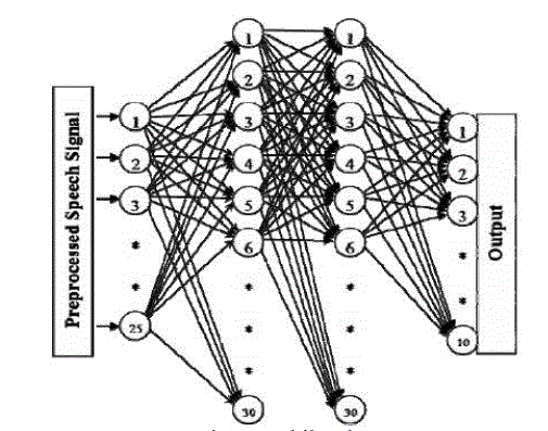
| An artificial neural network (ANN), often just called a neural network (NN), is an interconnected group of artificial neurons that uses a mathematical model or computational model for information processing based on a connectionist approach to computation. In most cases an ANN is an adaptive system that changes its structure based on external or internal information that flows through the network. The particular model used in this technique can have many forms, such as multi-layer perceptions or radial basis functions. The MLP is a type of neural network that has grown popular over the past several years. A MLP with one input layer, one hidden layer, and one output layer is shown in Fig.5. MLP’s are usually trained with an iterative gradient algorithm known as back propagation [10]. |
| The MLP is convenient to use for problems with limited information regarding characteristics of the input. However, the optimal MLP architecture (number of nodes, hidden layers, etc.) to solve a particular problem must be selected by trial and error, which is a drawback. In addition, the training time required to solve large problems can be excessive, and the algorithm is vulnerable to converging to a local minima instead of the global optimum. The MLP can be applied to speaker recognition [11] as follows. First, the feature vectors are gathered for all speakers in the population. The feature vectors for one speaker are labeled as “one” and the feature vectors for the remaining speakers are labeled as “zero.” An MLP is then trained for that speaker using these feature vectors. The MLP’s for all speakers in the population are trained using this method. In this paper, we have chosen to use a back propagation neural network [12, 13,14] since it has been successfully applied to many pattern classification problems including speaker recognition [15] and our problem has been considered to be suitable with the supervised rule. |
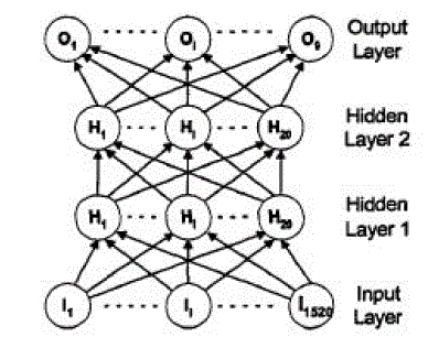
| MLP neural network we used consists of four layers; one input layer, two hidden layers and one output layer. The structure of the back propagation neural network is shown in Figure 6. The first layer has 1,520 input neurons (152 frames x 10 LPC-orders) which are fully connected to the first hidden layer. The two next hidden layers consist of 20 neurons per layer. The last layer is the output layer consisting of 9 neurons which one output neuron represented one speaker. All four layers are fully feed forwarded. |
| B. HIDDEN MARKOV MODEL (HMM) |
| The Hidden Markov Model (HMM) is a variant of a finite state machine having a set of hidden states Q, an output alphabet (observations) O, transition probabilities A, output (emission) probabilities B, and initial state probabilities II. The current state is not observable. Instead, each state produces an output with a certain probability (B). Usually the states Q, and outputs O, are understood, so an HMM is said to be a triple (A, B, II). |
| Description of HMM |
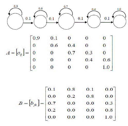
| For the description figure 7 shows an example of Hidden Markov Model, The model consists of a number of states, shown as the circles in figure. At time t the model is in one of these states and outputs an observation (A, B, C or D) [16] [17]. At time t+1 the model moves to another state or stays in the same state and emits another observation. The transition between states is probabilistic and is based on the transition probabilities between states which are given in state j at time t+1. Notice that in this case A is upper triangular. While in a general HMM transitions may occur from state to any other state, for speech recognition applications transitions only occur from left to right i.e. the process cannot go backwards in time, effectively modeling the temporal ordering of speech sounds. Since at each time step there must always be a transition from a state to a state each row of A must sum to a probability of 1. The output symbol at each time step is selected from a finite dictionary. This process is again probabilistic and is governed by the output probability matrix B where Bjk is the probability of being in state j and outputting symbol k. Again since there must always be an output symbol at time t, the rows of B sum to 1 [18]. Finally, the entry probability vector π is used to describe the probability of starting in described by the parameter set λ = [π, A, B] |
| A HMM is characterized by the following: |
| 1) N, the number of states in the model. The individual states are denoted as S={S1,S2,….,Sn} and the system state at time t as q1. |
| 2) M, the number of distinct observation symbols per state, i.e. the discrete alphabet size. The individual symbols are denoted as V = {v1,v2,….,vm} |
3) The transition probability distribution A={aij} where, each aij is the transition probability from state Si to state Sj. Clearly,  |
4) The observation symbol probability distribution B = bjk where, each bjk is the observation symbol probability for symbol vk, when the system is in the stae Sj.  |
| 5) The initial state distribution π={ π } where, π = P[q1 = S1], 1 ≤ j ≤ N. HMM model can be specified as λ = (A,B, π,M,N,V). In this thesis, HMM is represented as λ = (A, B, π) and assume M, N and V to be implicit. |
| C. DYNAMIC TIME WARPING (DTW) |
| The Dynamic Time Warping (DTW) distance measure is a technique that has long been known in speech recognition community. It allows a non-linear mapping of one signal to another by minimizing the distance between the two. Dynamic Time Warping is a pattern matching algorithm with a non-linear time normalization effect. It is based on Bellman's principle of optimality [19], which implies that, given an optimal path w from A to B and a point C lying somewhere on this path, the path segments AC and CB are optimal paths from A to C and from C to B respectively. The dynamic time warping algorithm [12] creates an alignment between two sequences of feature vectors, (T1, T2,.....TN) and (S1, S2,....,SM). A distance d(i, j) can be evaluated between any two feature vectors Ti and Sj. This distance is referred to as the local distance. In DTW the global distance D(i,j) of any two feature vectors Ti and Sj is computed recursively by adding its local distance d(i,j) to the evaluated global distance for the best predecessor. The best predecessor is the one that gives the minimum global distance D(i,j) at row i and column j: |
 |
| The computational complexity can be reduced by imposing constraints that prevent the selection of sequences that cannot be optimal [20]. Global constraints affect the maximal overall stretching or compression. Local constraints affect the set of predecessors from which the best predecessor is chosen. Dynamic Time Warping (DTW) is used to establish a time scale alignment between two patterns. It results in a time warping vector w, describing the time alignment of segments of the two signals. assigns a certain segment of the source signal to each of a set of regularly spaced synthesis instants in the target signal. |
| D. VECTOR QUANTIZATION (VQ) |
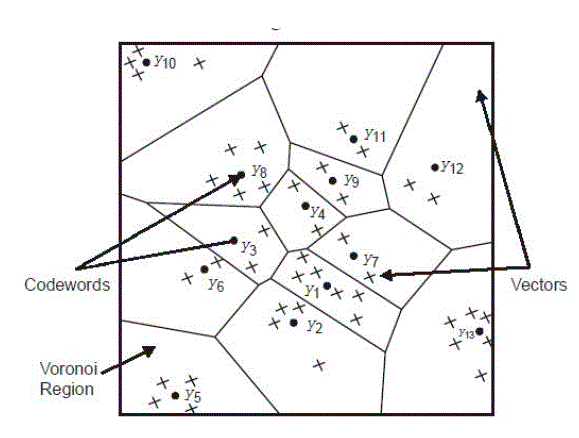
| Vector Quantization is the classical quantization technique from signal processing which allows the modeling of probability density functions by the distribution of prototype vectors. It works by dividing a large set of points into groups having approximately the same number of points closest to them. Each group is represented by its centroid point. The density matching property of vector quantization is powerful, especially for identifying the density of large and high-dimensioned data. Since data points are represented by the index of their closest centroid, commonly occurring data have low error, and rare data high error. Hence, Vector Quantization is also suitable for lossy data compression. |
| A vector quantizer maps k-dimensional vectors in the vector space Rk into a finite set of vectors Y = {yi : i = 1, 2,..., N}. Each vector yi is called a code vector or a codeword and the set of all the code words is called a codebook. Associated with each codeword, yi, is a nearest neighbor region called Voronoi region, and it is defined by: Vi = {x ÃâÃâ Rk : || x – yi || < || x – yj ||, for all j ≠ 1}. Given an input vector, the codeword that is chosen to represent it is the one in the same Voronoi region. |
The representative codeword is determined to be the closest in Euclidean distance from the input vector. The Euclidean distance is defined by:  |
| where xj is the jth component of the input vector, and yij is the jth is component of the codeword yi. |
| E. GAUSSIAN MIXTURE MODEL (GMM) |
| The Gaussian mixture model (GMM) is a density estimator and is one of the most commonly used types of classifier. In this method, the distribution of the feature vector x is modeled clearly using a mixture of M Gaussians. |
 |
| Here μi, Σi represent the mean and covariance of the ith mixture. Given the training data x1, x2…xn, and the number of mixture M, the parameters μi, Σi, ai is learn using expectation maximization. During recognition, the input speech is again used extract a sequence of features x1, x2…xL... the distance of the given sequence from the model is obtained by computing the log likelihood of given sequence given the data. The model that provides highest likelihood score will verify as the identity of the speaker. A detailed discussion on applying GMM to speaker modeling can be found in [22]. |
V. COMPARATIVE RESULT ANALYSIS
|
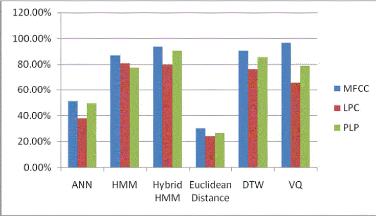
| We have compared the result of different classifiers with the feature extraction techniques MFCC, LPC, and PLP feature extraction techniques. In an average the MFCC and VQ techniques give the maximum recognition rate. We have shown the recognition percentage of different classifier with different feature extraction techniques in table 1. Figure 9 shows the graph of recognition of speech. |
VI. CONCLUSION
|
| This paper has illustrated the different feature extraction and classifier techniques of speaker identification through experimental research. MFCC is well known techniques used in speaker recognition to describe the signal characteristics, relative to the speaker discriminative vocal tract properties. The goal of this review was to create a speaker recognition system, and apply it to a speech of an unknown speaker. By investigating the extracted features of the unknown speech and then compare them to the stored extracted features for each different speaker in order to identify the unknown speaker. |
Tables at a glance
|
 |
| Table 1 |
|
| |
Figures at a glance
|
 |
 |
 |
 |
 |
| Figure 1 |
Figure 2 |
Figure 3 |
Figure 4 |
Figure 5 |
| |
 |
 |
 |
 |
| Figure 6 |
Figure 7 |
Figure 8 |
Figure 9 |
|
| |
References
|
- Campbell J.P. and Jr. “Speaker recognition: A Tutorial” Proceeding of the IEEE. Vol 85, 1437- 1462 1997.
- S.Furui. “Fifty years of progress in speech and speaker recognition,” Proc. 148th ASA Meeting, 2004.
- A. Rosenberg, “Automatic speaker recognition: A review,” Proc. IEEE, vol. 64, pp. 475487, Apr.1976.
- G. Doddington, “Speaker recognition-Identifying people by their voices,” Proc. IEEE, vol. 73, pp. 1651-1664, 1985
- R.KlevansandR.Rodman, “Voice Recognition, Artech House, Boston, London 1997.
- Corneliu Octavian DUMITRU, Inge GAVAT, “A Comparative Study of Feature Extraction Methods Applied to Continuous Speech Recognitionin Romanian Language”, 48th International Symposium ELMAR-2006, 07-09 June 2006, Zadar, Croatia.
- DOUGLAS O’SHAUGHNESSY, “Interacting With Computers by Voice: Automatic Speech Recognition and Synthesis”, Proceedings of theIEEE, VOL. 91, NO. 9, September 2003, 0018-9219/03 2003 IEEE.
- A.P.Henry Charles &G.Devaraj, “Alaigal-A Tamil Speech Recognition”, Tamil Internet 2004, Singapore.
- N.UmaMaheswari, A.P.Kabilan, R.Venkatesh, “A Hybrid model of Neural Network Approach for Speaker independent Word Recognition”,International Journal of Computer Theory and Engineering, Vol.2, No.6, December, 2010 1793-8201.
- A. Dempster, N. Laird, and D. Rubin, "Maximum likelihood from incomplete data via the EM algorithm," J. Royal Stat. Soc., vol. 39, pp. 1-38,1977.
- D. E. Rumelhart and J. L. McClelland, Parallel Distributed Processing. Cambridge, MA: MIT Press, 1986.
- J. Oglesby and J. S. Mason, “Optimization of neural models for speaker identification,” in Proc. ICASSP, 1990, pp. 261-264.
- L Fausette, "Fundamentals of Neural Networks- Architecture, Algorithm, and Applications", Prentice Hall, 1994.
- SNNS (Stuttgart Neural Network Simulator) User Manual, Version 4.1, University of Stuttgart, Institute for Parallel and Distributed HighPerformance Systems (IPVR), Report No. 6/95 W. Sintupinyo, P. D~bey, S. Sa-tang, V. Thailand, p. 238-246, March-April 1999.
- Y.-Yan, M. Fanty, and R. Cole, "Speech Recognition Using Neural Networks with Forward-backward Probability Generated Targets",Proceedings of International Conference on Acoustics, Speech, and Signal Processing, Munich, April 1997.
- Rabiner, L. and Wilpon, J. and Soong, F. (1988), “High Performance Connected Digit Recognition using Hidden Markov Models”, IEEETransaction of Acoustic, Speech, and Signal Processing, Vol. 37, No. 8, pp. 1214-1225.
- Rabiner, L. and Levinson, S. (1989), “HMM Clustering for Connected Word Recognition”, in proceedings of International Conference onAcoustic, Speech and Signal Processing (ICASSP), Glasgow, UK, Vol. 1, pp. 405-408.
- Rabiner, L. and Levison, S. (1985), “A Speaker-independent, Syntax-Directed, Connected Word Recognition System based on Hidden MarkovModel and level building”, IEEE Transactions on Acoustics, Speech and Signal Processing, Vol. 33, Issue 3, pp. 561-573.
- R. Bellman and S. Dreyfus, “Applied Dynamic Programming”. Princeton, NJ: Princeton University Press, 1962.
- H. Silverman and D. Morgan, “The application of dynamic programming to connected speech recognition” IEEE ASSP Magazine, vol. 7, no. 3, pp. 6-25, 1990.
- Om PrakashPrabhakar and Navneet Kumar Sahu, “A Survey On: Voice Command Recognition Technique” IJARCSSE,Volume 3, Issue 5, May2013.
- Reynolds, D. A. and Rose, R. C. "Robust text-independent speaker identification using Gaussian mixture speaker models. IEEE Trans. SpeechAudio Process. 3, 1995, pp 72–83.
- LohMun Yee Abdul Manan Ahmad, “Comparative Study of Speaker Recognition Methods:DTW, GMM and SVM” Malaysia Skudai, 81310Johor DarulTa’zim, Malaysia.
- Vimala.C and Dr.V.Radha, “A Review on Speech Recognition Challenges and Approaches” World of Computer Science and InformationTechnology Journal (WCSIT) ISSN: 2221-0741 Vol. 2, No. 1, 1-7, 2012.
|