Research & Reviews: Journal of Ecology and Environmental Sciences
ISSN: 2347-7830
ISSN: 2347-7830
Uche E. Uche*
Department of Mechanical Engineering, Air Force Institute of Technology, Kaduna, Nigeria
Received: 21-Sep-2023, Manuscript No. JEAES-23-114402; Editor assigned: 25-Sep-2023, Pre QC No. JEAES-23-114402 (PQ); Reviewed: 09-Oct-2023, QC No. JEAES-23-114402; Revised: 16-Oct-2023, Manuscript No. JEAES-23-114402 (R); Published: 23-Oct-2023, DOI: 10.4172/2347-7830.11.4.001
Citation: Uche EU. Evaluation of Hydrologic Data for Irrigation System Design: A Case Study. RRJ Ecol Environ Sci.2023;11:001
Copyright: © 2023 Uche EU. This is an open-access article distributed under the terms of the Creative Commons Attribution License, which permits unrestricted use, distribution, and reproduction in any medium, provided the original author and source are credited.
Visit for more related articles at Research & Reviews: Journal of Ecology and Environmental Sciences
The scope and the efficient operation of an irrigation system depend on systematic collection, collation, and analysis of the hydrological/meteorological data of the project area. Relying on existing rainfall records, the peak rainfall, mean rainfall, rainfall frequency and effective monthly rainfall were established. Atayi stream discharge characteristic curve was used to determine the stream stage-discharge relationship while the instantaneous rate of discharge of the stream was determined using float. The generated data was plotted on a hydrograph to obtain 2.64 m3/s. The high-level volume discharge and the low-level flow per annum were found to be 29.08 m3 and 18.33 m3 respectively. For the crop evapotranspiration, the Penman open water evaporation was deployed using climatic data for Igwu scheme as collected by Umudike Research Institute, Umuahia to obtain 1871 mm per annum compared to 2200 mm by Piche or Pan evaporation. The site hydrologic data collected and analyzed supports the adequacy of basic hydrologic factors for irrigated paddy rice cultivation in the study area.
Discharge; Effective; Penman; Piche; Evapotranspiration
The ultimate success of every water resource project depends on the correct assessment of availability of water on which the size of the project is determined [1]. Since design is concerned with future events whose time or magnitude cannot be certain, resort is often made to statements of probability or frequency in the design of engineering systems. When there is an insufficient amount of data, simple analysis techniques can often yield statistically acceptable predictions of events [2]. Evaporation from an open water surface is often estimated from inadequate data and relationship between this and crop water requirement may be transposed from one area or even country whose climate bears only a superficial resemblance to that of the area under study. Such is the nature of engineering system design that a sound knowledge of hydrologic concepts is today a pre-requisite. The design of irrigation and drainage system basically requires three hydrologic information: (1) Rainfall; (2) Water supply and (3) Crop consumptive use. The hydrological information on rainfall comprises such terms as annual series, partial duration, and probability of occurrence intervals. Dalrymple described the annual series as a group of annual extremes and the partial duration series as being made up of all large events above a given base [3]. Linsley and Frezini defined it as the recurrence of an event of specified magnitude and of an equal or larger magnitude [4]. Recurrence Interval can be estimated from equation 1 [2].
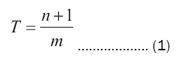
Where,
T=Recurrence interval (yr.)
n=Number of years of record
m=Position of event in the series, highest being one.
The annual series interval is the average interval in which event of a given size is likely to reoccur as an annual maximum. The recurrence interval of the partial duration series is the average interval between events of a given size regardless of their relation to the year or any other time period [5]. For an event having a recurrence interval of T, the probability that it will be equaled or exceeded in any one year is obtained from equation 2.
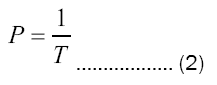
Where,
P=Probability of recurrence
T =Return period (year).
Kessler and Raad after a thorough study of the accuracy of the various approaches to forecasting future event objected to the use of the annual series on the basis that the second highest event in some years may exceed the maximum events recorded in other years, resulting in under-estimation of events of short-term periods [6]. They further recommended the use of the partial duration series for agricultural purposes. On their part Linsley and Frezini opined that partial duration series be used to determine the frequency of rare events [4]. They further observed that it is particularly useful where lesser event and recurrence interval less than a year, are of interest. On his part, Schwab noted that the annual and partial duration series give essentially identical results for periods greater than 10 years [7]. The knowledge of the rate of water-use by crops is fundamental in the design of the water supply system and scheduling of irrigation scheme. The pattern of crop water use, allowing for rainfall and operational losses determines the canal, pipeline, storage, and pumping capacities of system [8]. The consumptive use of water by crop includes not only the moisture transpired by the plants and that used in the building of plant tissue but also the water evaporated from the plant foliage and from the soil on which the crop is growing. It is influenced by climate factors especially temperature, length of growing season, and to a lesser extent humidity of the air and wind movement [9]. The most used method for calculating evapotranspiration under humid conditions is that of Penman. In Penman formula the evaporation for an open water surface is calculated from combined heat balance thermodynamic equations, utilizing measurements of air temperature and humidity, run of wind and number of hours of bright sunshine. The equation 3 used is:
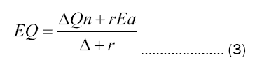
In which,
EQ=Evaporation from open water surface mmH2O/dy
Δ=Slope of saturation vapour pressure Vs temperature curve (mmHg per°C)
Qn= Net radiation (mmH2O/day)
r=Reflection co-efficient of evaporation surface (0.06)
Estimate of the crop evapotranspiration is obtained by multiplying the value obtained (the evaporation) by the crop coefficient (K). This ranges from 0.6 to 0.8 depending on the month [10]. The equation has since been modified as follows:
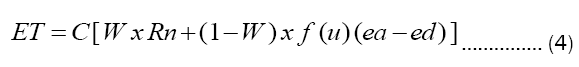
Where,
ET=Reference evapo-transpiration (mm/dy)
W=Temperature–related weighting factor
Rn=Net radiation in equivalent evaporation (0.25 mm/dy for most crops)
f (U)=Wind related function
(ea-ed)=Difference between the saturated vapour pressure at mean air temperature and the mean pressure of the air (bars).
C=Adjustment factor to compensate for the effect of day and night weather conditions.
This modification became necessary to remove certain Penman constants which doubtably are thought to vary from one climate to another [5]. The prediction model is based on climatological data which can be divided into three common methods [7].
• Mass transfer–moisture moves away from evaporation and transpiring surfaces in response to the combined phenomena of turbulent mixing of pressure gradient.
• Energy balance-heat is required for the evaporation of water so if there is no change in a water temperature then the net radiant or heat supplied is a measure of evaporation [11].
• Empirical methods–energy available for evaporation is proportional to the temperature.
On these grouping Jensen observed that all three involve empirical relationships to some extent since even the combined Penman equation utilizes an empirical wind function as shown in equation 5 [12].
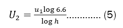
Where,
U2=wind speed at 2 meters height (mpd)
U1=wind speed at any other height (mpd)
h=any other height (feet)
Important too is that the crop co-efficient is dependent upon the maturity of the crop and soil moisture status. As soil moisture tension increases plants are not always able to extract sufficient water from the root zone to satisfy the potential evapotranspiration. At such time, although water requirements are reduced the plants may become temporarily wilted and produce lower yields [2]. The study is to examine the quantity, quality, time distribution and annual variation of the hydrologic features of a paddy rice project site to ascertain its dependability for year-round rice cultivation under irrigation as a guide for irrigation system design.
Study site
The study site is the fairly level swamp valley of Atayi stream which includes the flood plain of Iyioma and Mbuka, occupying about 16 hectares out of the 169.55 ha swamp field (Figure 1). It is a rainfall swamp that is flooded during the rainy season by run off from the surrounding uplands and rainfall on the swamp surface. The two combined, is more than the restricted natural drainage channel through the swamp can carry. The valley is mainly uncultivated and uncleared. Forest cover varies from heavy to light. However, some fields outside the high flood area are under rice cultivation mainly on rainfed basis without artificial drainage or structure for water level control. The rice grows well but yields are low, because of poor water control, low fertilizer use and low-potential rice variety.

Figure 1: Topographic map of study site.
Ground water exist often in unconfined condition with the water table tending southward to the coast. The depth of water table in the region is about 122 m below the ground surface [13].The most current bore holes record (for water supply is Ibina village) indicate the following in Table 1 as:
| Bore hole A | Bore hole B | |
|---|---|---|
| Total depth | 135 m | 108 m |
| Casing depth | 108 m | 85.5 m |
Table 1. Current bore holes record.
At the pump station where these data were collected no information on hydraulic conductivity, porosity, permeability, compressibility, Storability, transmissivity etc. were available.
Rainfall record verification
The test allows the reliability of rainfall records to be evaluated. It involves the subtraction of the mean rainfall for the year of record from the first year of record, leaving a sub-total, addition of the sub-total to second year of record and again the subtraction of the mean leaving a second sub-total. The process is continued to the end of the record. The sub-totals are then plotted against time. If a rainfall record is consistent there is a definite trend in the plotted points [14].
Determination of time distribution and annual variation of rainfall
The only meteorological station within the study area is sited at Igwu World Bank Irrigation Project where only a few years of records are available. To supplement this short record, data from Umudike 48 km from the area have been combined with the Igwu records to give 16 years (sixteen years) continues record for the period between 1968 and 1983. Umudike data have been used from 1968 to 1978 and Igwu for the remaining period (Table 2).
| Air temp (o C) | Relative humidity % | Wind speed | Piche evaporation (mm) | Rainfall (mm) | |
|---|---|---|---|---|---|
| Jan | 26.1 | 60 | 330 | 31.2 | |
| Feb | 27.3 | 70 | 370 | 15.58 | |
| Mar | 27.2 | 75 | 320 | 97.04 | |
| Apr | 27.5 | 80 | 260 | 194.18 | |
| May | 27 | 79 | 140 | 314.9 | |
| Jun | 25.5 | 83 | 110 | 303.02 | |
| Jul | 25.5 | 84 | 100 | 380.78 | |
| Aug | 25.7 | 85 | 90 | 159.9 | |
| Sep | 26.2 | 83 | 110 | 410.72 | |
| Oct | 26.2 | 81 | 90 | 244.58 | |
| Nov | 27.2 | 71 | 120 | 30.2 | |
| Dec | 26 | 62 | 160 | 1.6 |
Table 2. Summary of mean monthly climate factors.
Because of the war which affected Umuahia in 1969 the reliability of 1969-1970 record is questionable. Hence only the June records was extracted for the purpose of this analysis. This period is critical to crop growth in the proposed farm. Two empirical methods were used to estimate the part of the mean monthly rainfall that could contribute to meet the crop water requirement. The first method developed by U.S. Bureau of Reclamation involves a reduction factor which determines the rainfall that is effective based on total monthly rainfall amount [15]. The second method involves the estimation of effective rainfall using table prepared by the United States Department of Agriculture. To determine the peak rainfall-amount, the annual and the partial duration series were employed.
Determination of quantity of irrigation water supply
The main source of water supply for the project irrigation water need is the Atayi stream which drains directly into the Igwu river and forms part of the Igwu river basin. The Iyioma stream is not considered important in this analysis as it is not perennial. To estimate the instantaneous quantity of water available in the Atayi stream, float test was carried out in the stream to obtain the average velocity. The cross-sectional area of the flow was determined and multiplied with the velocity of flow to determine the discharge. This was plotted on a hydrograph against time from which the area under the curve gave the total volume of water discharged.
Determination of Atayi river water quality
Analysis of Atayi stream water was carried out in the water resource laboratory of Department of Civil Engineering University of Nigeria, Nsukka to ascertain the suitability of the Atayi water for irrigation purposes [16]. The chemical characteristics of particular interest if the water is to be used for irrigation include sodium absorption ratio and water conductivity value. The test was carried out according to the procedures outlined in the standard methods for the examination of water [17].
Crop water use
The value of evaporation from open water surface, potential evapotranspiration or reference crop evapotranspiration was obtained by Penman methods and modified or adjusted to apply to the crop of interest to obtain the consumptive use.
Climate
The climate of Igbere, a town in which the study site is located does not differ from the rest of the rainforest belt of Southern Nigeria. In other words, Igbere enjoys a warm tropical climate with well-defined wet and dry season. It rains between April and October with a marked break in August and averages between 1500 and 2500 mm per annum. The temperature is high throughout the year with monthly mean of 26.60C [16]. A look at the mean record (Table 1) indicates a general lower temperature value for the months of June (26.0oC) July (25.50C) August (25.50 c) and September (25.70C) corresponding to the high storm of 303 mm in June, 381 mm in Jul, 411 mm in September and the low storm of 160 mm in August (due to the August storm break). The highest mean temperature for the month were recorded for February (27.30C), March (27.20C), and April (27.50C) all of which fall outside the temperature modifying harmattan periods of December and January, and the heavy storm periods of June, August, September, and October. Humidity in the region also follows similar pattern as rainfall and temperature being highest during the high storm months. High relative humidity prevails in the area except for December and January yet the value does not fall below 50%.
Rainfall
Record verification: Figure 2, plotted from Table 3, shows the rainfall record to be consistent over the record year with a definite trend of fall- rise–fall–rise. This, however, serves as a rough screen for reliability since the record year is too short and the method rough. A better method of rainfall test would have been the double–mass analysis which involves the accumulative plotting of one set of data against an already reliable record [2].

Figure 2: Test of rainfall record.
| Year | Rainfall (mm) | Mean (mm) | Sub-total (mm) |
|---|---|---|---|
| 1979 | 2091 | 2101.14 | 10.14 |
| 1980 | 2258.6 | 2101.14 | 147.32 |
| 1981 | 2042.4 | 2101.14 | 88.58 |
| 1982 | 2364.5 | 2101.14 | 351.94 |
| 1983 | 1769.2 | 2101.14 | 0 |
Table 3. Annual rainfall for Igbere (Source: Igwu Meteorological Station MANR).
| Year | Annual peak (mm) | Other peaks | Annual series (mm) | Partial duration series (mm) | Return interval (year) |
|---|---|---|---|---|---|
| 1979 | 325 | 322, 277, 248, 243, 240, 198 | 550 | 550 | 6 |
| 1980 | 486.67 | 331, 219.9, 339.4, 441.45 | 506 | 506 | 5 |
| 1981 | 437.6 | 250.4, 420, 421.2 311.6, 210 | 486 | 486 | 2 |
| 1982 | 536 | 218, 191.5, 437, 228, 250, 321 | 437 | 441.5 | 1.5 |
| 1983 | 550 | 236, 429, 166.2, 310 | 325 | 439 | 1.2 |
Table 4. Peak rainfall analysis of the study area.
Time distribution and annual variation of rainfall: To determine the peak rainfall-amount, the annual and the partial duration series are employed. Figure 3, which is plotted using Table 4, indicates a peak 10 yr. storm of 575 mm. A mean annual storm corresponding to the 2.33-year recurrence interval can be read to be 470 mm for the annual series and 485 for partial series.

Figure 3: Rainfall recurrence interval.
Rainstorm frequencies: Daily rainfall data for the combined Umudike and Igwu records was analyzed to calculate the frequencies of occurrences for duration of 1, 2, 3, and 5 days. Only the June record was extracted for the purpose of this analysis (Table 5).
| Month | Per 1 day (mm) | |||
| 100 | 75 | 50 | 25 | |
| June | 3 | 6 | 4 | 38 |
| Freq/Yr | 0.013 | 0.029 | 0.076 | 0.54 |
| Per 2 days (mm) | ||||
| 100 | 75 | 50 | 25 | |
| June | 0 | 4 | 6 | 10 |
| Freq/Yr | 0.13 | 0.19 | 0.3 | 1 |
| Per 3 days (mm) | ||||
| 100 | 75 | 50 | 25 | |
| June | 0 | 2 | 13 | 0 |
| Freq/Yr | 0.17 | 0.5 | 0.67 | 1 |
| Per 4 days (mm) | ||||
| 100 | 75 | 50 | 25 | |
| June | 0 | 1 | 3 | 0 |
| Freq/Yr | 0.11 | 0.44 | 0.56 | 0.1 |
| Per 5 days (mm) | ||||
| 100 | 75 | 50 | 25 | |
| June | 1 | 2 | 2 | 3 |
| Freq/Yr | 0.2 | 0.4 | 0 | 1 |
Table 5. Frequency of storm for the june month.
Rainstorm frequencies: Daily rainfall data for the combined Umudike and Igwu records was analyzed to calculate the frequencies of occurrences for duration of 1, 2, 3, and 5 days. Only the June record was extracted for the purpose of this analysis (Table 5).
This period is critical to crop growth in the proposed farm. For purpose of drainage system design, Wang, and Hagan, observed that there is significant increase of rice crop damage if submergence lasts three days or longer in the two-month period following transplanting [2]. Kessler et al, on choice of design frequency, considered average failure of only once in five or ten years adequate for agricultural purposes. Hence for the month of June, the two-day duration, and the ten years (10-year) recurrence interval which are the critical period, critical duration and design frequencies respectively are recommended for the purpose of the project drainage system design [6]. Recurrent interval for 3–day duration cannot be extrapolated on available extreme paper sheet (Table 6 and Figure 4).

Figure 4: Storm frequency curve.
| Probability of occurrence (%) | Return period (yrs) | Rainfall (mm) | ||||
|---|---|---|---|---|---|---|
| Duration | ||||||
| 1 day | 2 day | 3 day | 4 day | 5 day | ||
| 10 | 10 | 145 | 250 | 245 | ||
| 20 | 5 | 125 | 205 | 240 | 195 | |
| 25 | 4 | 115 | 190 | 225 | 175 | |
| 40 | 2.5 | 95 | 165 | 195 | 170 | |
| 50 | 2 | 70 | 155 | 295 | 180 | 160 |
Table 6. Rainfall amounts for duration 1, 2, 3, 4 and 5 days for selected probabilities.
Effective rainfall: Two empirical methods were used to estimate the part of the mean monthly rainfall that could contribute to meet the crop water requirement (Table 7). The first method developed by U.S. Bureau of Reclamation involves a reduction factor which determines the rainfall that is effective, based on total monthly rainfall amount [15,18]. However, Dastane considered the method more suited to arid region [19].
| Total monthly precipitation that might occur (mm) | Monthly precipitation considered | |
|---|---|---|
| Part of each increment | Accumulated total | |
| mm | mm | |
| 25.4 | 24.13 | 24.13 |
| 50.8 | 22.86 | 46.99 |
| 76.2 | 20.86 | 67.82 |
| 101.6 | 16.51 | 84.33 |
| 127 | 11.43 | 95.76 |
| 12.4 | 6.35 | 102.11 |
Table 7. Incremental and accumulated effective monthly rainfall.
The second method involves the estimation of effective rainfall using table prepared by the United States Department of Agriculture. From total rainfall and monthly consumptive use, effective values for the rainfall amount were computed (Table 8).
| Months | Mean monthly rainfall (mm) | Effective rainfall based on USBR method (mm) | Effective rainfall based on USDASCS method (mm) |
|---|---|---|---|
| Jan | 31.2 | 29.14 | 19.24 |
| Feb | 15.8 | 15.58 | 9.6 |
| Mar | 97.04 | 84.91 | 44.26 |
| April | 194.18 | 104.2 | - |
| May | 314.9 | 110.2 | 47.54 |
| June | 303.02 | 109.65 | 95.07 |
| July | 380.78 | 113.53 | 97.53 |
| Aug | 159.88 | 102.48 | 92.61 |
| Sept | 410.72 | 115.02 | 72.94 |
| Oct | 244.58 | 106.72 | - |
| Nov | 30.2 | 28.69 | 18.33 |
| Dec | 1.6 | 1.6 | 1.31 |
Table 8. Effective rainfall determined by two different methods.
The more conservative result for the effective rainfall obtained using the United State Department of Agriculture, Soil Conservation Service (USDASCS) method is adopted because it considered most of the factors influencing crop water use by relating recorded rainfall, and crop evapotranspiration to irrigation depth. [9]. The effective rainfall obtained by the above methods must differ for different crops and soil types. As Wang and Hagan noted, rainfall occurrence and hence effective rainfall is probalistic in nature [2]. Therefore, a more reliable analysis of rainfall and its effectiveness for crop production should be based on statistical analysis. Unfortunately, all the necessary input data for such analysis are not available for the project locality.
Irrigation water supply
The main source of water supply for the project irrigation water need is the Atayi stream which drains directly into the Igwu and forms part of the Igwu river basin which is seen in Figure 1. The Atayi stream runs across the field dividing it into two unequal parts with the land rising gently on either side. It covers over 800 m within the project area, takes a land width of about 6.5 m and cuts into the soil to a depth of well over 3.5 m. This section examines the quantity, time distribution, annual variation, and dependability of the Atayi perennial stream as the main source of irrigation water supply to the project.
Atayi water quantity: The identification of viable farm irrigation system alternatives requires a knowledge of the available flow rate during the irrigation season. Hence the flow rate during the irrigation season was determined and result is as shown in Tables 9 and 10.
| Section | Depth (m) | Width (m) | Length (m) | Time (s) | Area (m2) | Flow velocity. (m/s) | Discharge rate (m3/s) | Discharge Vol (m3) |
|---|---|---|---|---|---|---|---|---|
| 1 | 1.01 | 1.5 | 4.2 | 18 | 1.52 | 0.23 | 0.35 | 6.4 |
| 2 | 2.18 | 1.5 | 4.2 | 16 | 3.27 | 0.26 | 0.86 | 13.7 |
| 3 | 2.29 | 1.5 | 4.2 | 15 | 3.44 | 0.28 | 0.96 | 14.4 |
| 4 | 1.13 | 1.5 | 4.2 | 15 | 1.7 | 0.28 | 0.47 | 7.1 |
| Total | 1.65 | 1.5 | 4.2 | 16 | 2.48 | 0.26 | 0.65 | 10.4 |
Table 9. Atayi stream flow test using float.
| Month | Highest | Lowest | Maximum discharge | Minimum discharge |
|---|---|---|---|---|
| (m) | (m) | m3/s | m3/s | |
| Jan | 0.94 | 0.92 | 1.51 | 1.48 |
| Feb | 1.01 | 0.83 | 1.63 | 1.34 |
| Mar | 1.16 | 0.88 | 1.87 | 1.42 |
| Apr | 1.22 | 0.88 | 1.96 | 1.42 |
| May | 1.72 | 0.9 | 2.77 | 1.45 |
| Jun | 1.77 | 0.97 | 2.85 | 1.56 |
| Jul | 2.18 | 0.97 | 3.51 | 1.56 |
| Aug | 2 | 1.18 | 3.22 | 1.9 |
| Sept | 2.29 | 1.21 | 3.69 | 1.95 |
| Oct | 2.18 | 0.98 | 3.51 | 1.82 |
| Nov | 2.18 | 0.98 | 3.51 | 1.58 |
| Dec. | 0.97 | 0.88 | 1.56 | 1.42 |
Table 10. Atayi stream stage–discharge relationship.
This volume is, however, not constant as it depends on the peak and the time interval.
From Figure 5 the high-level volume discharge of the Atayi stream is 29.08 m3 and the low level 18.33 m3 flow per annum when plotted on a hydrograph.
Table 11 shows that in 1976 the difference between the peaks flow rate 2.95 m3/s in September and lowest flow rate of 1.57 m3/s in January was as much as 1.38 m3/s, while in 1977 it was about 1.45 m3/s, 1978 about 1.58 m3/5 1979 about 1.63 m3/5 while the 1980, 1981, and 1982 had ranges of about 1.51 m3/s 2.07 m3/s and 1.88 m3/s respectively.

Figure 5: Atayi stream discharge rate.
| Year/Month | 1976 | 1977 | 1978 | 1979 | 1980 | 1981 | 1982 |
|---|---|---|---|---|---|---|---|
| Jan | 1.57 | 1.59 | 0.98 | 1.12 | 1.65 | 1.33 | 1.99 |
| Feb | 1.63 | 1.72 | 0.97 | 1.37 | 1.49 | 1.34 | 1.89 |
| Mar | 1.68 | 1.63 | 1.11 | 1.67 | 1.59 | 1.51 | 2.31 |
| Apr | 1.84 | 1.73 | 1.17 | 1.36 | 2.07 | 1.51 | 2.14 |
| May | 1.68 | 1.7 | 3.07 | 2.01 | 2.25 | 2.26 | 2.79 |
| June | 2.33 | 1.2 | 1.42 | 2.9 | 2.46 | 1.8 | 3.33 |
| July | 1.93 | 2 | 2.12 | 2.44 | 2.95 | 2.52 | 3.77 |
| Aug | 1.26 | 2 | 2.69 | 2.5 | 2.79 | 3.58 | |
| Sep | 2.95 | 2.17 | 2.29 | 2.75 | 2.51 | 3.41 | 3.3 |
| Oct | 2.87 | 2.47 | 2.5 | 2.47 | 2.68 | 2.96 | 3.54 |
| Nov | 2.43 | 1.51 | 1.63 | 1.71 | 1.94 | 2.36 | 2.62 |
| Dec | 1.5 | 1.02 | 1.14 | 1.67 | 1.47 | 1.99 |
Table 11. Computed mean monthly discharge of Atayi stream.
If the instantaneous rate of discharge in a river is plotted on a hydrograph against time, the area under the curve represents the total volume of water discharged. This volume is however a function of both peak and other discharges as well as the time interval considered and should therefore not be considered constant. The volume of water available in Atayi stream varies from month to month as the climate passes through the yearly cycle. Also, the volume of water available in any given month varies from year to year.
Atayi levels: The Atayi stream is situated at an altitude of about 115 m above sea level in the village of Amaiyi in Igbere. The volume of water retain in the stream varies between 29 m3 and 18 m3 with a depth that fluctuate between 2.72 m and 0.58 m over the year. Minimum and maximum monthly levels of the Atayi stream have been recorded by the Ministry of Agriculture and Natural Resources, Owerri over a period of only seven years (1975-1982). In this analysis the annual extreme values were plotted using Table 12 in Figure 6.

Figure 6: Frequency analysis of Atayi stream monthly peak and levels.
| Year | Annual peak monthly level (m) | Annual series | Return period |
| 1976 | 2.65 | 2.72 | 8 |
| 1977 | 2.16 | 2.65 | 4 |
| 1978 | 2.15 | 2.5 | 2.67 |
| 1979 | 2.3 | 2.3 | 2 |
| 1980 | 2.72 | 2.16 | 1.6 |
| 1981 | 2.5 | 2.15 | 1.33 |
| 1982 | 1.82 | 1.82 | 1.14 |
Table 12. Atayi high levels and plotting position (annual series).
For the design of pump station, it was decided to select a design level which had a return period in excess of 30 years. From a frequency distribution of monthly peak values, the 30 year return period at Atayi was calculated. The design stream level of 3.6 m for a 30-year return period was obtained (Figure 6).
With a bed level of 95.25 m the high-water level would then be 99.35 m. This level is about 0.88 m above the highest recorded during the data period. It was therefore considered that a design level of 99.40 m is satisfactory for sitting in the pumping house. The mean low levels recorded in the Atayi stream were shown in Table 10 and the frequency plot of monthly return annual low values obtained from Figure 7. A straight line was visually fitted to the annual series of the low levels to obtain the 30 years stream level of 0.475 m. This gave a stream level of 96.23. This value is about 0.11 m below the minimum water depth recorded during the 8-year record period.

Figure 7: Frequency analysis of Atayi stream monthly low levels.
Table 13 shows the theoretical distribution of the return periods. From the table a 30-year return period with 50% assurance level would yield a 21-year interval.
| Year | Annual minimum (m) | Annual series (m) | Return period year |
|---|---|---|---|
| 1976 | 0.63 | 0.58 | 8 |
| 1977 | 0.62 | 0.62 | 4 |
| 1978 | 0.58 | 0.63 | 2.67 |
| 1979 | 0.67 | 0.67 | 2 |
| 1980 | 0.86 | 0.77 | 1.6 |
| 1981 | 0.77 | 0.86 | 1.33 |
| 1982 | 0.95 | 0.95 | 1.14 |
Table 13. Atayi stream low levels and plotting position.
In this analysis the return periods quoted for the design levels of the pumping station and the abstraction level are considered conservative. This is however justified on the grounds that the records chosen in the analysis were limited to actual recorded data and too short to be relied upon. Further the recurrence interval computed by equation 1 are estimated average return periods and there is no implication that such floods will occur at even reasonably constant intervals [20].
Atayi stream water quality: The Atayi stream water is found fit for irrigation purposes. However, because of changes in water chemistry and soil condition that would develop from irrigation, routine monitoring of the water quality is recommended [16].
Crop water use
The Penman estimates (Table 14) were calculated using the longer record at Umudike. Position of Umudike lat. 08 o 29 ‘N long 07 033 ’E Attitude 120 m (Table 14).
| Jan | Feb | Mar | Apr | May | Jun | Jul | Aug | Sep | Oct | Nov | Dec | |
|---|---|---|---|---|---|---|---|---|---|---|---|---|
| Air temperature oC | 25.6 | 27.4 | 28.3 | 28 | 26.9 | 25.7 | 25.7 | 25.7 | 26.4 | 27 | 27 | 26.9 |
| Relative humidity % | 61 | 69 | 75 | 81 | 82 | 85 | 86 | 85 | 82 | 81 | 72 | 64 |
| Wind speed (mi/dy) | 72 | 48 | 58 | 58 | - | 70 | 29 | 34 | 32 | - | 31 | 31 |
| Mean monthly sunshine | 5.5 | 6.8 | 5.5 | 5.6 | 5.7 | 4.5 | 3.2 | 2.9 | 2.7 | 4.4 | 5.3 | 6..2 |
| Radiation rate | 13.9 | 14.8 | 15.4 | 15.1 | 14.7 | 14.9 | 15.2 | 15.3 | 14 | 13.7 |
Table 14. Summary of mean monthly climatic factors for the penman open water evaporation [21].
Table 15 is a summary of Penman open water surface evaporation compared with similar information in the region.
| Month | Penman EO (mm) | Piche EO | Computed |
|---|---|---|---|
| (mm) | Pen EO (mm) | ||
| Igwu stream | Igwu rice scheme design value | ||
| (1979 – 1983) | |||
| Jan | 99 | 330 | 190 |
| Feb | 117 | 370 | 180 |
| Mar | 68 | 320 | 193 |
| Apr | - | 260 | 172 |
| May | 64 | 140 | 160 |
| Jun | 108 | 190 | 150 |
| Jul | 95 | 100 | 119 |
| Aug | 108 | 90 | 130 |
| Sep | 99 | 110 | 120 |
| Oct | - | 90 | 140 |
| Nov | 123 | 120 | 142 |
| Dec | 128 | 160 | 175 |
| Total | 2200 | 1871 |
Table 15. Comparison of open water evaporation by various methods.
Olivier cautioned that the formula estimates are intended to be used for forecasting average requirement for design purposes and not as an operating formula for individual year unless there is otherwise reasonable confidence for a particular locality concerning the capacity of the soil unit on one hand to deal with surplus rates of precipitation, and on the other hand that the plant could draw on such soil storage [22]. Stanhill in evaluating the accuracy of meteorological estimates from the Penman observed that it gives too low estimate during harmattan and dry season months compared to the meteorological estimate of evapo-transpiration obtained during tank readings at Ibadan. Thornthwaite formula followed the same pattern while the radiation method utilized a lower proportion of incident solar energy during the late “summer” and “autumn” months. He however noted that the values obtained using the Penman formula gave excellent results for the annual totals but shorter records did not agree with measured values though they were correlated. Olivier however, posited that Piche evaporimeter does not present free water surface condition [23]. The World Bank Project Team used the Christiansen formula to obtain the “computed” pan evaporation. A check of the results shows marked difference in monthly surface evaporation obtained by the various methods. However, a discernible pattern of dry season, high evaporation and wet season, low evaporation are common to all.
The study set out to generate, evaluate and present basic hydrologic data for a rice paddy irrigation system design as a case study. The process and results of such study serve as a guide for the design of irrigation system. Although the Penman method is seen to underestimate evaporation under low air humidity such as during the harmattan months, particularly when compared with Pans or Piche Evaporation, the method is satisfactory for the conditions that apply around and within the project perimeter due to presence of large water surfaces. The air passing over large irrigation schemes (including the world bank rice project at Igwu) and numerous water surfaces during the harmattan will certainly be modified to increase the humidity. Penman open water surface evaporation is adopted. Its applicability to Nigeria humid region has been studied by Stanhill and found satisfactory. Finally, it is worthy of note that the water velocity obtained in this study is not necessary the mean velocity of flow as the float is aided by wind requiring modification of result by some constant. The site hydrologic data collected and analyzed however, support the adequacy of basic hydrologic factors for irrigated paddy rice cultivation in the study area.