Michael Engler*
Department of Business Administration and Engineering, Furtwangen University, Furtwangen, Germany
Received: 17-Nov-2023, Manuscript No. JSMS- 23-120358; Editor assigned: 20-Nov-2023, Pre QC No. JSMS- 23-120358 (PQ); Reviewed: 04-Dec-2023, QC No. JSMS- 23-120358; Revised: 11-Dec-2023, Manuscript No. JSMS- 23-120358 (R); Published: 18-Dec-2023, DOI: 10.4172/RRJ Stats Math Sci. 9.4.001
Citation: Engler M. Fast Numerical Simpson and Boole Integration by Using the Derivatives at the Boundaries. RRJ Stats Math Sci.2023.9.001.
Copyright: © 2023 Engler M. This is an open-access article distributed under the terms of the Creative Commons Attribution License, which permits unrestricted use, distribution, and reproduction in any medium, provided the original author and source are credited.
Visit for more related articles at Research & Reviews: Journal of Statistics and Mathematical Sciences
This article shows the extension of the closed Newton-Cotes numerical integration of Simpson’s and Boole’s rule by using the odd derivatives of the function at the boundaries of the integration interval. The derivatives can be used to efficiently increase the convergence order of numerical integration and a fast decrease of the error. Furthermore, due to its simplicity, it is very easy to write into program code, which is also shown. The error estimation is given and proven. Also, the method is confirmed with two different examples for numerical integration, of π and of the integral of the Gaussian distribution. Here, the method is compared to some common numerical integration methods, showing comparably faster convergence.
Numerical integration; Numerical quadrature; Derivative-based quadrature; Closed newton-cotes integration; Quadrature error estimation MSC Classification: 65D30, 65D32
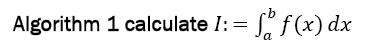
Given a function Supposed one wants to calculate the integral
 and a primitive of f is not known, does not exist in closed form or is too difficult to be calculated. Then, numerical calculation methods are needed, one of which is presented here. A very good comprehension of the different methods is given by Davis and Rabinowitz [1]. For numerical integration as presented here, the interval [a,b] is dissected into n equidistant intervals of width h:
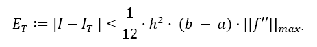
There are n+1 x- values, denominated a= x0,x1,.....xn-1,xn=b Within each interval, f is approximated by an interpolation function which is then integrated instead of f. The results of each approximated intervals are summed over all intervals and give an approximate solution of the integral. When h → 0, the numerical solution approaches the real value of the integral. One of the simplest numerical integration schemes is the Trapezoidal Quadrature. Here, the value IT of the numerical integration is calculated to:
with the error ET being of the order 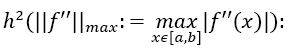
When one uses not only the function values, but also the values of its derivatives, the convergence order and speed strongly improves. It is already known that the use of the first derivative at the boundaries a and b lead to an increase of convergence order byh2 [1]. The method is known as the Euler-MacLaurin summation formula [2]. This approach is also shown in different characteristics from Ujevic and Catinas et al [3,4]. Davis, Rabinowitz and Stancu and Stroud have shown that the integral of the function f can be approximated by the function values and the values of arbitrary derivatives of the function [5]. Here, the derivatives at all nodes are used for the calculation. This method has been detailed by Burg and Burg and Degny [6,7]. They give the error estimations for different Newton-Cotes quadrature rules in combination with the first, second and third derivative and they show that both the convergence order increases and the error decreases in these cases.
In this article, we show that when using Newton-Cotes Quadrature in combination with any odd derivative of f at the boundaries, the convergence order vastly increases and the error decreases with each derivative being used. One great advantage of the odd derivatives is that only the derivatives at the boundaries are needed. We give the Simpson Quadrature formula extended with any odd derivative and its error estimation, showing that the error is of the order h2m+4, where m is the highest number of the odd derivative being used (m=1, first derivative, m=2, third derivative, and so on). Furthermore, the error coefficient decreases vastly with every higher derivative being used. The same holds for the extended Boole Quadrature formula, where the error is of the order h2m+6. Both algorithms, which are very easy to implement, are given.
Simpson Quadrature with Odd Derivatives
The Trapezoidal Quadrature can be extended by using not only two function values per interval, but by interpolating multiple intervals with values of different weights. These methods lead to the well-known Newton-Cotes formulas, e.g. Simpson’s rule and Boole’s rule. Details are shown in any textbook of basic numerical mathematics, e.g. Simpson’s rule is given by using two combined intervals and three values [2]:
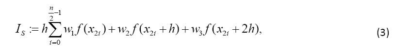
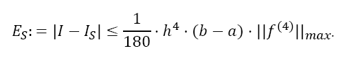
with the weights 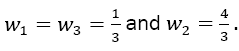 The error of Simpson’s rule is converging by the order of h4 two orders of magnitude faster than that of the Trapezoidal rule. The error coefficient is decreased by a factor of 15 (1/180 compared to 1/12):
Definition of Simpson Odd Derivative
We will now extend the classical Simpson rule by the odd derivatives at the borders, giving the so-called "Simpson Odd Derivative Quadrature SOD” in Table 1.
Definition 1 (Simpson Odd Derivative Quadrature SOD): Given the integral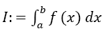 and the Simpson Rule defined by Equation 3 with n even and equidistant dissections of the interval of width h (defined by Equation 1) of the function
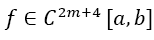 , with a natural number m ≥ 1. Given also the odd derivatives of f at the borders with
  with at least one
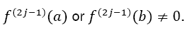
A fast converging formula for the numerical value of the integral is then calculated by:
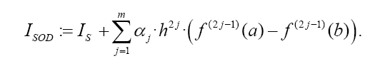
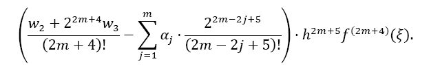
The weights w1 differ compared to Equation 3 with the number of derivatives m being used. They are shown together with the αj in Table 1. We will now calculate the coefficients given in Table 1. For this, we will approximate f by its Taylor series up to the degree 2m + 3 within the interval iranging from xi to xi+ 2h. Then follows:
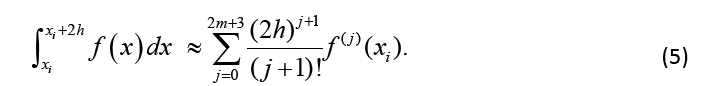
Using the definition of ISOD , Equation 4, and considering only the interval from xi to xi+ 2h, the Taylor approximation up to the degree 2m+ 3 gives:

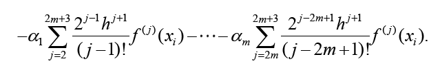
Adding all n/2 intervals ISOD,itogether gives the approximation of ISOD . Note that only the leftmost and rightmost derivatives remain, as the inner derivatives cancel each other out. This works only when the odd derivatives are used, when even derivatives are used, the inner derivative values remain and the method will become much less efficient. For the calculation of the optimal w1,w2,w3 and α j , Equation 5 and Equation 6 have to be set equal, as only then the approximation SOD gives the integral approximation. Comparing the coefficients with the corresponding derivatives, the following LSE with 4 + 2m rows and 3 + mcolumns results:
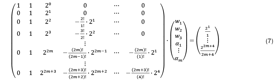
Although the LSE has more rows than variables, the solution is unique (without proof) and gives the coefficients w1, w2, w3, and αj, for the Simpson-Odd-Derivative Quadrature formula, Equation 4. The values when using the first five odd derivates ( m= 5) have been and are shown in Table 1. Higher derivatives can be calculated from Equation 7, but the calculation becomes more awkward due to the small numbers where one has to take care about rounding errors.
Please note again, that only the odd derivatives at the borders of the interval are needed and with each odd order being added, the convergence is by order of 2 faster. Additionally, the error coefficient γ decreases strongly, as will be shown below. Please note that in the case of the method is still applicable but not so effective. Overall, the method is applicable when
 ∞ and it becomes more efficient when the higher derivatives of f are not becoming too large with higher orders.
The quadrature ISOD is “optimal” in the sense that the approximation is perfect for any polynomial p(x) being of maximum degree 2m + 3. This means that |I − ISOD |= 0 for  This directly follows from the calculation formula given now, and needs thus not be proven.
Error estimation
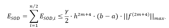
Theorem 1 (Error estimation of Simpson Odd Derivative): The quadrature error of the Simpson Odd Derivative Integration is of the order h2m+4:

With the error coefficient γ given in Table 1.
Proof: Considering the quadrature error, one has to calculate the Taylor error. The Taylor remainder of order 2m + 4 of Equation 5 is 
The remainder of Equation 6 is:
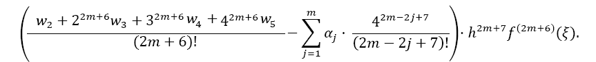
The overall error ESOD,ifor one interval ifrom xito xi +2m is then calculated by the difference of both Taylor remainders:
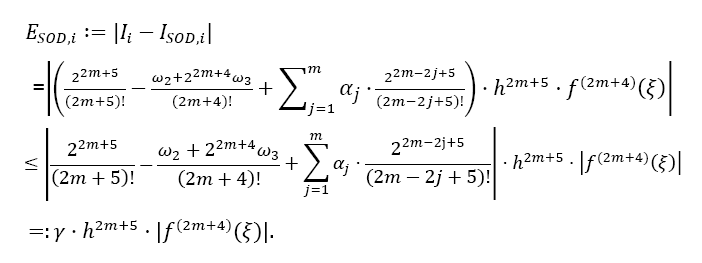
This gives the calculation for the error coefficient γ . Please note from Table 1, that the factor γ decreases about a factor of 40 for each higher odd derivative used (this factor seems to converge to 4π2 ≈ 39, 48 for higher derivatives, likewise for the Euler- MacLaurin formula, but this is just an assumption) !
| m | w1=w3 | w2 | α1 | α2 | α3 | α4 | α5 | Error coef. γ |
|---|---|---|---|---|---|---|---|---|
| 1 |  |
 |
 |
 |
||||
| 2 |  |
 |
 |
 |
 |
|||
| 3 |  |
 |
 |
 |
 |
 |
||
| 4 |  |
 |
 |
 |
 |
 |
 |
|
| 5 |  |
 |
 |
 |
 |
 |
 |
 |
Table 1. Coefficients of the simpson odd derivative quadrature up to m=5 (9th derivative).
For the overall error then holds, using Equation 1:
Boole Quadrature with Odd Derivatives
When one uses not two neighbouring intervals but four, the quadrature formula referred to Boole results. For this, the integral of f can be calculated by:

With the weights 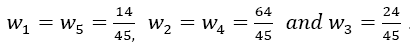 The error of Boole’s rule is converging by the order of h6, two orders of magnitude faster than Simpson’s rule:
Definition of Boole Odd Derivative
Like for the Simpson rule, Boole’s rule can also be extended by the odd derivatives at the borders, leading to the socalled “Boole Odd Derivative Quadrature BOD”.
Definition 2 (Boole Odd Derivative Quadrature BOD): Given the integral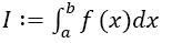 and Boole’s Rule IB defined by Equation 9 with n doubly even and equidistant dissections of the interval of width h (defined by Equation 1) of the function
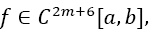 with a natural number m ≥ 1. Given also the odd derivatives of f at the borders with
 with at least one
 or
or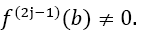
A fast converging formula for the numerical value of the integral is then calculated by:
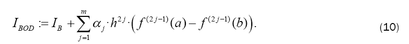
The weights wi differ compared to Equation 9 with the number of derivatives m being used. They are shown together with the αj in Table 2. The result for m = 1 is also given by Burg in [6]. In this paper we give a general approach for any odd derivative used.
The approach to calculate the wiand αj is identical to SOD, but the numbers slightly change. This time, f is approximated by its Taylor series up to order 2m + 5. When using the same approach as in Equations 5 and 6 with the Taylor series up to order 2m + 5, the following LSE with 6 + 2m rows and 5 + m columns results:
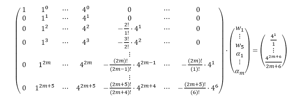
The solution of the LSE gives the coefficients wi and αjof Table 2. The error of BOD is zero for all polynomials of degree smaller or equal to 2m+ 5.
| m | w1=w5 | w2=w4 | w3 | Îñ1 | Îñ2 | Error coef. Îó |
|---|---|---|---|---|---|---|
| 1 |  |
 |
 |
 |
 |
|
| 2 |  |
 |
 |
 |
 |
 |
Table 2. Coefficients of the boole odd derivative quadrature up to m=2 (third derivative); due to numerical instabilities, the calculation of the LSE for m âÃâ°ÃÂ¥ 3 is not practical).
Error estimation
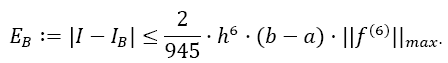
Theorem 2 (Error estimation of Boole Odd Derivative): The quadrature error of the Boole Odd Derivative Integration is of the order h2m+6:
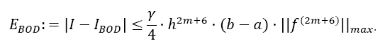
With the error coefficient γ given in Table 2.
Proof: The proof is analogous to the proof for SOD. In this case, the Taylor remainder of order 2m+6 has to be considered. The remainder for the integral I from xi to xi + 4h is (xi ≤ξ≤ xi + 4h):
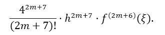
The remainder of Equation 10 is:
The overall error ESOD,i for one interval i from xi to xi + 4h is calculated by the difference of both Taylor remainders:
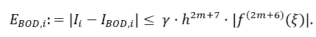
The error coefficient γ then calculates to:
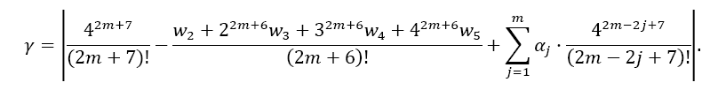
Here, also, the error coefficient decreases by a factor of about 40 with each odd derivative being used.
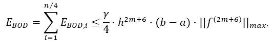
The overall error then is, using Equation 1:
Applications
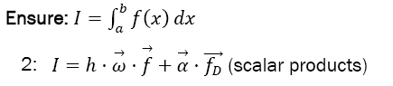
Algorithm: In the following we give the algorithm. It has to be noticed that the algorithm is practical, when the derivatives of f at the borders are easy to calculate, which is usually provided in common programming languages like Python, Mathematica or Matlab. Then, the derivatives at the borders have to be calculated only once and the integral is easily calculated to any accuracy needed. The main advantages are its simple calculation and its very fast convergence. However, when the derivatives of f are not easy to be determined or its values at the borders become excessively large, the algorithm may not be suited.
Require:
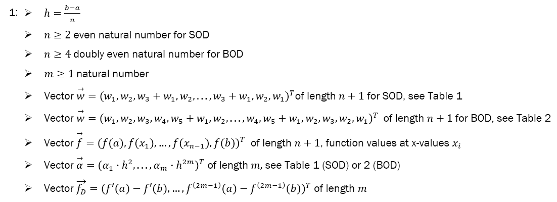
Please note that only SOD or BOD needs to be chosen. The algorithm (both SOD and BOD) uses in sum 3n + m2 + 8m + 5 operations, out of which are m + 1 + 2m function calls.
Example 1: Calculation of the Integral of the Gaussian distribution: Now we discuss the approximation of the integral of the Gaussian distribution with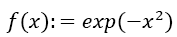 by Simpson and Boole Odd Derivative Quadrature and compare it with several common quadrature methods. In special, we calculate the integral by using Algorithm 1.
Results for the absolute error of Simpson Odd Derivative Quadrature over step size and number of operations are given in Figure 1. One clearly sees three effects:

Figure 1: Absolute error of  over step width h (left image) and the number of operations (right figure) using Simpson Odd Derivative (Equation 4).
→ The much faster convergence of SOD compared to the normal Simpson Quadrature without derivatives,
→ The much more efficient convergence of SOD, especially when using higher derivatives; machine precision accuracy is given within about 100 operations or only 16 steps (h= 0.125),
→ The overall very small errors especially for decreasing interval size h.
When comparing SOD with BOD as given in Figure 2, one sees that Boole Odd Derivative is even more efficient than Simpson Odd Derivative, but the effect is not as strong as expected, showing about a one order of magnitude smaller error with the same number of intervals or operations. However, the effect of the derivatives is evident, as each derivative decreases the error by about a factor of 100, two orders of magnitude.

Figure 2: Absolute error of over step width h. (left image) and the number of operations (right figure) using Simpson and Boole Odd Derivative up to m=2.
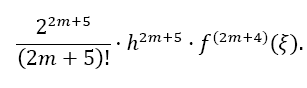
To further classify the method, we compare it with usual Newton Cotes Quadratures. For this, we calculate I:=  up to an accuracy <1e-12. We show how many operations and function calls are necessary to reach this accuracy. As methods we use the Trapezoidal, Simpson and Boole Quadrature without derivatives and SOD and BOD up to m=3. Table 3 shows the results. The efficiency of the use of odd derivatives can clearly be seen. Take e.g. SOD with m=3. According to Table 1 and Equation 4, the error estimation for m=3 (5th derivative) depending on the step width h is

which leads to a very small error even at a relatively large step width (or small numbers of n). Additionally, very little numbers of operations and function calls are necessary, resulting in a very fast calculation.:
Example 2: Calculation of π : As indicated above, the strength of the method shows especially when both the number of derivatives m and the number of intervals n is increased, which means that the width h is decreased. For the second illustration, we take the function f(x)=4/(1+x2). The primitive of the function is 4 arctan x, so for the integral from 0 to 1 follows:
This function fulfills all drawbacks concerning the method given above: the higher derivatives are hard to calculate by hand, so the prerequisites are not optimal. Furthermore, the higher derivatives at b increase extremely fast
 However; these drawbacks are highly compensated when one uses more intervals. Results are shown in Figure 3, which clearly show the very fast convergence towards π , even when using only the first and third derivative. Surprisingly, Boole Odd Derivative performs even less than Simpson Odd Derivative, probably coming from the ill conditions of the higher derivatives used for BOD.
| Rule | Degree m | Intervals n | Abs. error | #op | Function calls |
|---|---|---|---|---|---|
| Trapezoidal Rule (Eq. 2) | 0 | 155700 | 9.84E-13 | 311400 | 155700 |
| Simpson’s Rule (Eq. 3) | 0 | 506 | 9.93E-13 | 1520 | 507 |
| Boole’s Rule (Eq. 9) | 0 | 60 | 7.54E-13 | 185 | 61 |
| SOD (Eq. 4) | 1 | 36 | 8.43E-13 | 122 | 39 |
| SOD (Eq. 4) | 2 | 24 | 3.34E-13 | 97 | 29 |
| SOD (Eq. 4) | 3 | 12 | 8.83E-13 | 74 | 19 |
| BOD (Eq. 10) | 1 | 32 | 5.50E-13 | 106 | 33 |
| BOD (Eq. 10) | 2 | 16 | 7.50E-13 | 73 | 21 |
Table 3. Approximation of  to an accuracy <1e-12

Figure 3: Absolute error of over step width h (left image) and the number of operations (right figure) using Simpson and Boole Odd Derivative up to m=2.
In this paper, a very efficient and fast converging Quadrature formula for numerical integration has been shown, which is also very easy to implement. Besides of the function value, it also uses the odd derivatives of the function at the borders only. A general method for the calculation of several Newton-Cotes formulas with odd derivatives has been given, which is applicable to all Newton-Cotes Quadratures and shown here only for Simpson’s and Boole’s rule. With each odd derivative additionally used, the convergence increases with the square of the step size h2 and the absolute error coefficients decrease by about a factor of 40. The error formulas and a method to calculate the errors have also been given, with the error formula being proven.
The algorithm of the method has been given with all its prerequisites. It is very easy to write into program code. The efficiency of the algorithm has been shown using two common examples. Comparing it with usual Newton-Cotes formulas, a much faster convergence is shown, making the method very feasible. However, the method is not suitable in occasions when the derivatives of the function to be integrated are difficult or intricate to calculate. In any other cases, a very practical method is provided.
The code for the algorithm written in Python is available from the author.
The author likes to thank all Python enthusiasts and especially Guido van Rossum for that wonderful programming language.