International Journal of Advanced Research in Electrical, Electronics and Instrumentation Engineering
ISSN ONLINE(2278-8875) PRINT (2320-3765)
ISSN ONLINE(2278-8875) PRINT (2320-3765)
Rahana Fathima1 and Raseena P E2
|
| Related article at Pubmed, Scholar Google |
Visit for more related articles at International Journal of Advanced Research in Electrical, Electronics and Instrumentation Engineering
Digital processing of speech signal and voice recognition algorithm is very important for fast and accurate automatic voice recognition technology. The voice is a signal of infinite information. A direct analysis and synthesizing the complex voice signal is due to too much information contained in the signal. Taking as a basis Mel frequency cepstral coefficients (MFCC) used for speaker identification and audio parameterization, the Gammatone cepstral coefficients (GTCCs) are a biologically inspired modification employing Gammatone filters with equivalent rectangular bandwidth bands. A comparison is done between MFCC and GTCC for speaker identification.Thier performance is evaluated using three machine learning methods neural network (NN) and support vector machine (SVM) and K-nearest neighbor (KNN). According to the results, classification accuracies are significantly higher when employing GTCC in speaker identification than MFCC.
Keywords |
| Feature extraction, Feature matching, Gammatone Cepstral coefficient, Speaker identification |
INTRODUCTION |
| The speaker recognition has always focused on security system of controlling the access to control data or information being accessed by any one. Speaker recognition is the process of automatically recognizing the speaker voice according to the basis of individual information in the voice waves. Speaker identification is the process of using the voice of speaker to verify their identity and control access to services such as voice dialling, mobile banking, data base access services, voice mail or security control to a secured system. |
| The recognition and classification of audio information have multiple applications [1].The identification of the audio context for portable devices, which could allow the device to automatically adapt to the surrounding environment without human intervention [2]. In robotics this technology might be employed to make the robot interact with the environment, even in the absence of light, and there are surveillance and security system that make use of the audio information either by itself or in combination with video information [1]. |
PRINCIPLE OF VOICE RECOGNITION |
| A. Speaker Recognition Algorithms |
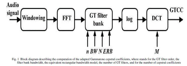
| A voice analysis is done after taking an input through microphone from a user. The design of the system involves manipulation of the input audio signal. At different levels, different operations are performed on the input signal such as Windowing, Fast Fourier Transform, GT Filter Bank, Log function and discrete cosine transform. |
| The speaker algorithms consist of two distinguished phases. The first one is training sessions, whilst, the second one is referred to as operation session or testing phase. |
| B. Gammatone Filter Properties |
| Gammatone function models the human auditory filter response. The correlation between the impulse response of the gammatone filter and the one obtained from the mammals was demonstrated in [3]. It is observed that the properties of frequency selectivity of the cochlea and those psychophysiclly measured in human beings seems to converge, since: 1) the magnitude response of a fourth-order GT filter is very similar to reox function [4], and 2) the filter bandwidth corresponds to a fixed distance on the basilar membrane. An nth-order GT filter can be approximated by a set of n firstorder GT filter placed in cascade, which have an efficient digital implementation. |
| C. Gammatone Cepstral Coefficients |
| Gammatone cepstral coefficients computation process is analogous to MFCC extraction scheme. The audio signal is first windowed into short frames, usually of 10–50 ms. This process has a twofold purpose 1) the (typically) nonstationary audio signal can be assumed to be stationary for such a short interval, thus facilitating the spectro-temporal signal analysis; and 2) the efficiency of the feature extraction process is increased [1]. Subsequently, the GT filter bank (composed of the frequency responses of the several GT filters) is applied to the signal’s fast Fourier transform (FFT), emphasizing the perceptually meaningful sound signal frequencies.1 Indeed, the design of the GT filter bank is the object of study in this work, taking into account characteristics such as: total filter bank bandwidth, GT filter order, ERB model (Lyon, Greenwood, or Glasberg and Moore), and number of filters. Finally, the log function and the discrete cosine transform (DCT) are applied to model the human loudness perception and decorrelate the logarithmiccompressed filter outputs, thus yielding better energy compaction. The overall computation cost is almost equal tothe MFCC computation [5]. |
 |
| D. Feature Extraction |
| The extraction of the best parametric representation of acoustic signals is an important task to produce a better recognition perfomance. The efficiency of this phase is important for the next phase since it affects its behavior. |
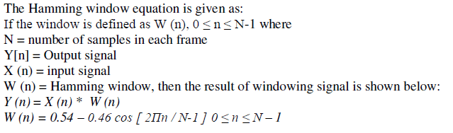
| Step 1: Windowing |
| The audio samples are first windowed (with a Hamming window) into 30 ms long frames with an overlap of 15 ms. The frequency range of analysis is set from 20 Hz (minimum audible frequency) to the Nyquist frequency (in this work, 11 KHz). This process has a twofold purpose 1) the (typically) non-stationary audio signal can be assumed to be stationary for such a short interval, thus facilitating the spectro-temporal signal analysis; and 2) the efficiency of the feature extraction process is increased. |
 |
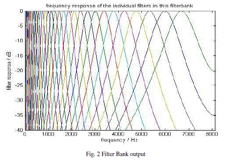
| Step 2: GT Filter Bank |
| The GT filter bank composed of the frequency responses of the several GT filters. It is applied to the signal’s fast Fourier transform (FFT), emphasizing the perceptually meaningful sound signal frequencies [5]. |
 |
| Step 3: Fast Fourier Transform |
| To convert each frame of N samples from time domain into frequency domain. |
| Y (w) = FFT [h (t) * X (t )] = H (w ) * X(w) |
| If X (w), H (w) and Y (w) are the Fourier Transform of X (t), H (t) and Y (t) respectively. |
| Step 4: Discrete Cosine Transform |
| The log function and the discrete cosine transform (DCT) are applied to model the human loudness perception and decorrelate the logarithmic-compressed filter outputs, thus yielding better energy compaction. |
METHODOLOGY |
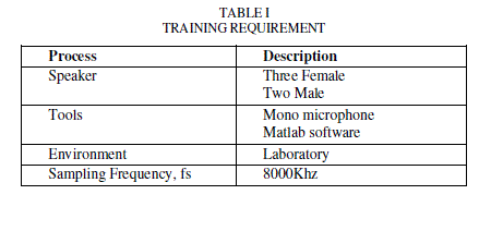
| Voice recognition works based on the premise that a person voice exhibits characteristics are unique to different speaker. The signal during training and testing session can be greatly different due to many factors such as people voice change with time, health condition (e.g. the speaker has a cold), speaking rate and also acoustical noise and variation recording environment via microphone [6]. Table I gives detail information of recording and training session. |
 |
EXPERIMENTAL EVALUATION |
| A. Audio Database |
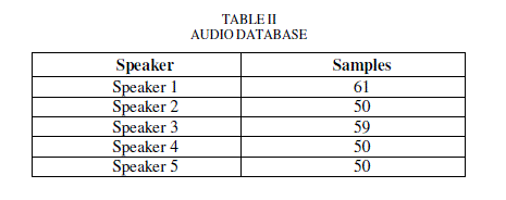
| Speech samples are taken from five persons. From each person 50 to 60 samples are taken .The length of the speech samples was experimentally set as 4s. |
 |
| B. Experimental Setup |
| The speech samples are first windowed (with a Hamming window) into 30 ms long frames with an overlap of 15 ms, as done in [7]. The frequency range of analysis is set from 20 Hz (minimum audible frequency) to the Nyquist frequency (in this work, 11 KHz). Subsequently, audio samples are parameterized by means of GTCC (both the proposed adaptation and previous speech-oriented implementations [4]–[8]) and other state-of-the art features (MFCC and MPEG-7). MFCC are computed following their typical implementation [9].With regard to MPEG-7 parameterization, we consider the Audio Spectrum Envelope (since it was the MPEG-7 low level descriptor attaining the best performance for non-speech audio recognition in which is converted to decibel scale, then level-normalized with the RMS energy [9], and finally compacted with the DCT. |
| Rather than performing the audio classification at frame-level, we consider complete audio patterns extracted after analyzing the whole 4 s-sound samples at frame-level. With reference to these kinds of sounds, it is of great relevance to consider the signal time evolution (including envelope shape, periodicity and consistency of temporalchanges across frequency chanels). Subsequently, the audio patterns obtained are compacted by calculating the mean feature vector over different intervals [8]. The main purpose of this process is to make the classification problem affordable without losing the feature space interpretability, which would happen if considering, for example, principal component analysis or independent component analysis [7]. This requirement is especially important, since we are mainly interested in determining the rationale behind the performance of GTCC in contrast to other state-of-the-art audio features. |
| Regarding the classification system, three machine learning methods are used for completeness: 1) a neural network (NN), and more specifically, a multilayer perceptron with one hidden layer; and 2) a support vector machine (SVM) with a radial basis function kernel and one versus all multiclass approach and K-nearest neighbor [8]. The audio patterns are divided into train and test data sets using a 10 10-fold cross validation scheme to yield statistically reliable results. Within each fold, the samples used for training are different from those used for testing. In addition, the last experiment employs a 4-fold cross validation scheme with a different setup, whose aim is to test the generalization capability of the features. The classification accuracy is computed as the averaged percentage of the testing samples co rectly classified by each machine learning method. |
EXPERIMENTAL RESULTS |
| A. GTCC Adjustment |
| The first experiment is conducted so as to adjust the GTCC computation for non-speech audio classification purposes. For each parameter (i.e., total filter bank bandwidth, GT filter order, ERB model, and number of filters), the value maximizing the classification accuracy is selected. Firstly, the positive effect of enlarging the filter bank bandwidth (with extensions both on the low and high frequencies) from the typical bandwidth employed in speech is demonstrated [9]. Secondly, the fourth, sixth, and eighth GT filter orders show very similar behavior. Among them, fourth-order filters are selected given their lower computational cost. Thirdly, it is observed that both Greenwood and Glasberg and Moore ERB models attain a better performance than Lyon’s. Between them, Glasberg and Moore are selected. Finally, N=48 filters are chosen, as a good trade-off between classification accuracy and filter bank complexity. |
| B. Features Comparison |
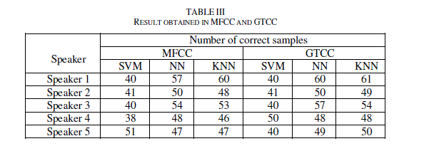
| In the following experiment, the proposed GTCC for the speacker recognition is done using three machine learning methods, neural network, support vector machine and K-nearest neighbor. GTCC and MFCC show comparable results when using the SVM. GTCC yielded a notably higher accuracy for both the KNN and the NN. |
 |
| C. Performance Comparison GTCC versus MFCC |
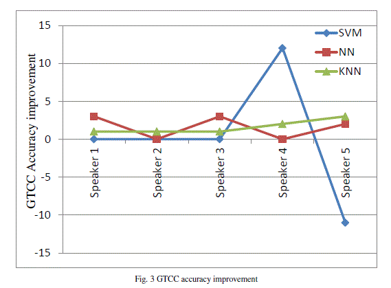
| Accuracy improvement yielded by GTCC with respect to MFCC is analysed. This improvement is calculated as the difference between the classification rates attained for each machine learning method. It should be noted that, in order to yield a fair comparison, the bandwidth of analysis (20 Hz-11 KHz), number of filters (48), and number of Cepstral coefficients (13) were identically set in both GTCC and MFCC. The GTCC performs notably better than the MFCC. Sounds like animals, birds show an important accuracy improvement. All sounds whose classification accuracy is improved when using GTCC share some spectral similarities, as they present particular components in the low part of the spectrum, i.e., below 1 KHz. |
 |
CONCLUSION |
| GTCC borrowed from the non-speech research field, have been adapted for the speaker identification. This paper has discussed voice recognition algorithm with three machine learning methods (Neural network, Support vector machine and K-nearest neighbor) which are important in improving the voice recognition performance. The technique was able to authenticate the particular speaker based on the individual information that was included in the voice signal. The results show that these techniques could be used effectively for voice recognition purposes. However, there is still room for further improvement through investigating the temporal properties of the audio signals, combining GTCC with other signal features and implementing the technique in real-time on multimedia portable devices. |
References |
|