Keywords
|
| ECG Signals, Polynoimal Approximation, Chebyshev Polynomials, Chebyshev Interpolation. |
INTRODUCTION
|
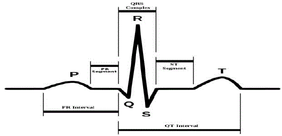
| Heart muscles produces electrical variations on the body of skin and the variations are measured by electrodes placed on specific positions on the body. These variations are referred to as ECG (Electrocardiogram) signals. From engineering point of view, an ECG signal is periodic. Figure 1 shows one cardiac cycle of the signal which is also known as the R-R interval with three indicated parts: P wave, QRS complex, and the T wave. These waves are the result of contraction and expansion of the heart muscles. The P wave is due to the depolarization of the atria whereas QRS complex reflects the rapid depolarization of the right and left ventricles. The T-wave represents the repolarization (or recovery) of the ventricles [1]. |
| The amount of data involved in storage and transmission of digital ECG signals is quite large. So it needs to be adequately compressed. The compression must be done in a way so that it can be accurately reconstructed. |
| The ECG compression techniques are broadly classified as: direct methods, transform-based methods and parameter extraction methods. In direct methods, the original ECG signal samples are compressed directly, and in transformation method the original samples are first transformed and then compressed. In parameter extraction methods, the features of the processed signal are extracted and then these features are used for the reconstruction of the signal [2]. |
| Various time domain compression algorithms for ECG signals can be found in the literature. These methods are based on the idea of extracting few significant signal samples to represent the signal and then decoding the same set of samples. The time domain algorithms are based on fast heuristics in the sample selection process. These techniques are faster but suffer from suboptimality. Examples of such techniques are the FAN algorithm [3] and the AZTEC algorithm [4]. Time domain algorithms were further improved by SLOPE [5] and AZTDIS [6] techniques. The Cardinality Constrained Shortest Path (CCSP) algorithm presented in [7] is based on a mathematical model of the entire sample selection process. Signal samples are modeled as nodes in a graph and then optimization techniques are applied for achieving higher compression ratio. |
| For ECG data compression, several compression algorithms including polynomial approximations and polynomial interpolation have been proposed. The advantage of polynomial approximation is that it requires only polynomial coefficients and it is able to approximate the original ECG signal quite efficiently. |
| Third order polynomials including splines have been used for ECG interpolation in [8] and [9]. ECG signals represented by second order quadratic polynomials were studied by Nygaard et. al. in [10]. Legendre polynomials of high degree were used for ECG data compression in[11], [12] and [13]. Generalized Jacobi polynomials were employed for ECG compression in [14]. Although Chebychev polynomials are widely used in mathematical interpolation and approximation, ECG signal compression through Chebychev polynomials are hardly found in the literature. In[15] ECG data compression is done using Discrete Chebyshev Transform by segmenting the signal into blocks which consist of multiple cardiac cycles. In [16] ECG signal data compression is done in the same way as in [15] but only significant Chebyshev coefficients are selected, transmitted and stored. |
| In this paper, we propose a computationally efficient method to model ECG signals through Chebyshev polynomials. In order to have a better compression ratio we must have a lower order of the polynomial. So we segment one complete cycle into various portions depending upon their structures. Next, we model each segment independently using Chebyshev interpolation and combine them to reconstruct the complete signal. |
| The rest part of the paper is organized as follows: in the next two sections, we give a brief introduction to Chebychev polynomials and Chebyshev interpolation. In section IV we describe the proposed method along with the algorithm to achieve ECG data compression. In section V we present the implementation of our method and discuss the results obtained. In the last section we give the conclusions. |
CHEBYSHEV POLYNOMIALS
|
| The Chebyshev polynomials of first type and degree n are defined in terms of trignometric cosine function as: |
 |
| The expressions for Chebyshev polynomials are obtained from the recursive relation |
 |
| The Chebyshev polynomials of degree n, Tn(x), has n zeros in the interval [-1, 1], which can be calculated as |
 |
| The roots of the Chebyshev polynomial are also known as Chebyshev points. In the same interval the n + 1 extrema of the polynomial Tn(x) are located at |
 |
| At all the maxima Tn(x) = 1, while at all the minima Tn(x) = -1. The Chebyshev polynomials are orthogonal in the interval [-1,1] over the weight w(x) = (1-X2)-1/2 . They also satisfy discrete orthogonality relationships. Other properties of Chebyshev polynomials can be found in [17]. |
POLYNOMIAL APPROXIMATION USING INTERPOLATION
|
| A polynomial approximation problem is of finding a polynomial close to a given function and has the freedom to select the significant points. Once the significant points have been fixed, it is reduced to an interpolation problem that can be solved by polynomial interpolation. Let y(x) represent ECG segment vector of length N consisting of samples of y(x) such that |
 |
| Given a set of N + 1 data points (xi,y(xi)) we want to construct a polynomial f of degree N with the property |
 |
| Suppose the interpolation polynomial is in the form |
 |
| which means that |
 |
| Substituting (6) in (5) we get a system of linear equations which in matrix form reads |
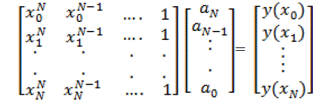 |
| The matrix on the extreme left is the Vandermonde's matrix. The system given by (7) would have a unique solution if the determinant of the Vandermonde matrix does not vanish. Solving this system for ak we can construct the interpolating polynomial f(x). |
| Alternatively we can write the required polynomial explicitly using Lagrange's formula as |
 |
| Let us now construct yet another interpolating polynomial p(x) by sampling f(x) at n interpolation points such that n < N. We can estimate the difference between them, i.e., the interpolation error E(x). Let ïÃÂÃÂn denote the space of polynomials of degree ≤ n, and let Cn+1[a, b] denote the space of functions that have n + 1 continuous derivatives on the interval [a, b]. Then we have this theorem: |
 |
| If we are free to choose the interpolating points x0 ,…, xn within this interval, then the product ïÃÂÃÂn j = (x-xj) can be minimized which in turn would minimize the interpolating error E(x). This can be achieved by choosing interval as [-1,1] and the interpolating points xj as the Chebyshev points. The following theorem gives an estimate of the error for the above case. |
| Theorem 2:Assume that p(x) interpolates f(x) at x0 , x1…, xn. Also assume that these n+1 interpolation points are the (n + 1) roots of the Chebyshev polynomial of degree Tn+1(x), which are given by (3).Then ïÃâ¬Ã¢x ε[-1,1], |
 |
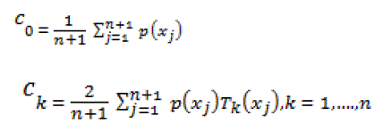
| Our goal is not to approximate a function p(x) on the interval [-1, 1] but to approximate the values of the function p(x) corresponding to the discrete set of points given by (3). An arbitrary function p(x) can be approximated in the interval [-1,1] by |
 |
| where the coefficients cj are defined as |
 |
PROPOSED METHOD
|
| Since we are processing one R-R interval, our working domain is in the interval [a, b]. So, we first transform the interpolation interval y ε[-1, 1] using |
 |
| This converts the interpolation problem for f(x) on [a,b] into an interpolation problem for f(x) = g(x(y)) in y ε[-1,1]. The Chebyshev points in the interval are y ε[-1, 1] the roots of the Chebyshev polynomial Tn(x), i.e., |
 |
| The corresponding n + 1 interpolation points in the interval [a, b] are |
 |
| The interpolation error is given by |
 |
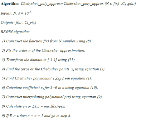
| In our method we need to construct the function f(x) using (8) with all the N ECG samples. Then we find the Chebyshev points and the Chebyshev interpolating polynomial using the nodes. Next we calculate the error and if the error is not within our tolerance we increase the order. We continue doing these operations till our error criterion is met. |
| Next we observe that to model the ECG signal over one R-R interval, the order of the Chebyshev polynomial may be quite high. So we segment the signal into various sections depending upon the structure of the section. Then we model each section independently using Chebyshev interpolation technique. |
| We present here an algorithm to show the steps of our method. |
| Algorithm Chebyshev_poly_approx=Chebyshev_poly_approx (N,ε , f(x) ,Ck ,p(x)) |
 |
SECTION RESULTS AND DISCUSSION
|
| An ECG signal is not linear, rather more curvaceous consisting of waves of various shapes. The proposed algorithm is implemented and tested over one R-R interval of the ECG signal. The performance of the Chebyshev approximation technique is measured by maximum absolute error and gridwise variation of error. |
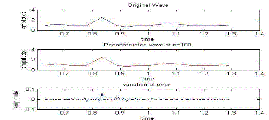
| For testing the performance of our algorithm we conducted our tests in MATLAB environment using a simulated standard ECG signal. The algorithm was initially applied over the R-R interval of the ECG signal. The signal consisted of 8274 samples and we fixed the error tolerance as ε = 10-2. To approximate one complete cycle we required Chebyshev polynomials upto order 100. The original and approximated signal with the error over one cardiac cycle is shown in Figure 2. |
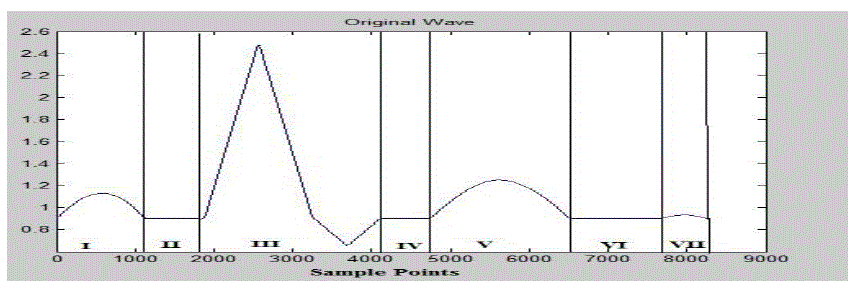
| Since the order of the Chebyshev polynomials is quite high and we needed a better compression, we segment the entire cycle into various sections. The shape and duration of the various waves of ECG is considered as the basis for segmentation. Therefore the number of sample points for different segments is different. All the seven segments of the complete cycle are shown in Figure 3. |
| The algorithm was applied over the sections and the order of Chebyshev polynomial was increased till the error was within the specified tolerance. |
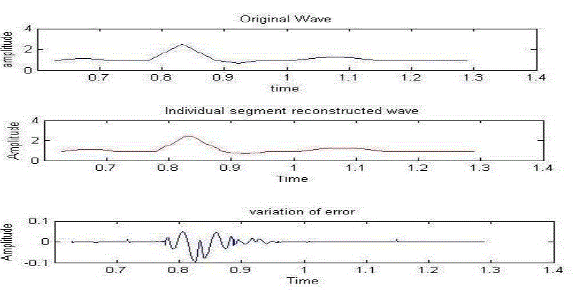
| The segmented original and the approximated signals along with the error over various segments is shown in Figure 4. Table I shows the variation of error with increasing order of the polynomials for different segments. It can be seen from the table that the segments with varying slopes require higher order as high as 8th order Chebyshev polynomials, whereas the segments where slope variations are less can be interpolated by Chebyshev polynomials with a maximum order of 3 within the specified error tolerance. |
| From Figure 3 and Table I it can be observed that the error for the section containing QRS complex is still quite high even for a 8 order polynomial (approximately 0.119). So this section is further segmented into three subsections. The error variation with increasing order of the approximated polynomials over different subsections are shown in Table II . |
| It can be seen from the table that the maximum absolute error is drastically reduced over the sections containing the QRS complex. Further it is observed that the individual subsections containing the QRS complex can be approximated with very low order polynomials. Error can also be reduced by further segmenting these subsections. |
CONCLUSION
|
| This paper proposes a technique to approximate simulated ECG signals using Chebyshev polynomials. Initially the complete signal over one cardiac cycle was approximated with higher order Chebyshev polynomials. The order of Chebyshev polynomials depends upon the shape of section ECG wave. Waves having zero or constant slope, can be approximated by lower order Chebyshev polynomials whereas waves having variable slopes require higher order Chebyshev polynomials. So various sections of simulated ECG were taken and approximated with comparatively lower Order Chebyshev polynomials. The approximation error can further be reduced by applying advanced segmentation techniques which would involve interval analysis. This work would be addressed as our future work. |
Tables at a glance
|
 |
 |
| Table 1 |
Table 2 |
|
Figures at a glance
|
 |
 |
 |
 |
| Figure 1 |
Figure 2 |
Figure 3 |
Figure 4 |
|
References
|
- Guyton, Textbook of Medical Physiology, 9th ed. Saunders W. H., 2010.
- M. Jalaleddine, C. G. Hutches, R. D. Strattan, and W. A. Cobberly, “ECG data compression techniques–a unified approach,” IEEETransactions on Biomed. Engg, vol. 37, no. 4, pp. 329–343, April 1990.
- L. Bohs and R. Barr, “Real-time adaptive sampling with the fan algorithm,” Medical and Biological Engineering and Computing, vol. 29,no. 6, pp. 565–573, 1988.
- J. R. Cox, F. M. Noelle, H. Fozzard, and G. Oliver, “Aztec a preprocessing program for real-time ecg rhythm analysis,” IEEE Transactionson Biomed. Engg, vol. 15, no. 2, pp. 128–129, April 1968.
- S. C. Tai, “Slope a real-time ecg data compressor,” Medical and Biological Engineering and Computing, vol. 29, no. 2, pp. 175–179,March 1991.
- S.C.Tai, “Aztdis a two phase real-time ECG data compressor,” Journal of Biomed. Engg., vol. 15, no. 6, pp. 510–515, Nov 1993.
- D. Haughland, J. Heber, and J. Husoy, “Optimisation algorithms for ecg data compression,” Medical and Biological Engineering andComputing, vol. 35, no. 4, pp. 420–424, July 1997.
- M. Karczewicz and M. Gabbouj, “ECG data compression by spline approximation,” Signal Processing, vol. 59, no. 1, pp. 43–59, 1997.
- M. Brito, J. Henriques, P. Carvalho, B. Ribeiro, and M. Antunes, “An ECG compression approach based on a segment dictionary and bezierapproximation,” Procedure EURASIP, vol. 15, pp. 2504–2508, sept 2007.
- R. Nygaard, D. Haughland, and J. Husy, “Signal compression by second order polynomials and piecewise non interpolating approximation,”Department of Electrical and Computing Engineering, Tech. Rep., 1999.
- W. Philips and G. Jonghe, “Data compression of ecg’s by high degree polynomials,” IEEE Trans on Biomedical Engineering, vol. 39, no. 4,pp. 330–337, April 1992.
- W. Philips, “Ecg data compression with time -warped polynomials,” IEEE Trans on Biomedical Engineering, vol. 40, no. 11, pp. 1095–1101,Nov 1993.
- A. A. Colomer and A. A. Colomer, “Adaptive ecg data compression using discrete legendre transform,” Digital Signal Processing, vol. 7,no. 4, pp. 222–228, Oct 1997.
- D. Tchiotsop, D. Wolf, V. Louisdorr, and R. Husson, “Ecg data compression using jacobi polynomials,” in IEEE Engineering in Medicine andBiology Society, vol. 2007, no. 29. Lyon France, 2007, pp. 1863–1867.
- D. Dchiotsop and I. S. Tlviu, “Ecg data communication using Chebyshev polynomial compression methods,” AsociatiaGenerala a Inginerilordin Romania, vol. 868, pp. 1–12, Dec 1990.
- F. Guendouzi and A. Mokhtari, “Polynomial modelling of the ecg signals,” Computer Medical Applications (ICCMA), vol. 1, pp. 1–5, 2013.
- G. Szego, “Orthogonal polynomials,” American Mathematical Society, vol. 23, pp. 38–57, 1975
|