Research & Reviews: Journal of Engineering and Technology
ISSN: 2319-9873
ISSN: 2319-9873
Biya Motto Frederic*
Department of Physics, Faculty of Sciences, University of Yaoundé I, P O Box 812, Cameroon
Received: 16/07/2014; Revised: 22/08/2014; Accepted: 27/08/2014
Visit for more related articles at Research & Reviews: Journal of Engineering and Technology
The article is devoted to diesel speed regular parametric tuning for training on ship simulator by means of MATLAB. To keep the controller as simple as possible PID regulator is used for step-response rising of quality indicators. For automated tuning the program in MATLAB codes is created. The example is considered
Simulator, ship diesel, parametric tuning, step response, transfer function, PID-controller.
The increase of requirements for energetic efficiency, safety and reliability of energetic installations in sea and waterway ships, on the basis of modern systems of automation and control is an important scientific and technical concern. The equipment supply of ships with complex technical means and systems, constructed with the new computer technologies, should be done simultaneously with the improvement in the level of professional training.
Efficient means of training such staffs are the simulators. In simulators and program complex at a good quality level, we solve problems of systems modelling, parametric tune with maximal approximation. We construct algorithms that permit us to avoid default situations. Simulators are widely used for research works, related to the choice of rational technical regimes and parametric optimisation of control systems with technical means in various applications.
For training of mechanical technicians, we can use simulators in machine sections [2]. In operating main ship motors and auxiliary mechanisms, we use control systems in simulators, equipped with regulators. We construct tune methods by various criteria. It has been proven by experience that the process of parametric tune and functioning characteristic optimisation of ship control systems have a certain volume of information in the simulator that is insufficient, for understanding the behaviour with feedback signals in statics and in dynamics. In the case where PID-regulators are corporate in automated systems, numerical values are recommended without convenient justification.
Further improvement in simulators can be done through construction of program simulators complexes, based on MATLAB/simulink medium. The principal advantage of MATLAB/simulink is that we can build various programs applied in different ships for navigation. The application of MATLAB assures high quality in modelling.
Modern technologies of modelling constitute an arsenal of efficient means for solving complex technical issues in waterways transport.
Let us solve a precise problem. We consider the analysis and modelling by MATLAB means of regulated automated system of rotation speed for a ship diesel. We do the parametric tune of PID-regulator to improve the control quality.
We note that the definition of parameters for PID-regulator tuning is one of the key problems for a simulator in machine section. The aim of modelling is to evaluate regulator properties of control system. The modelling object is the diesel equipment with shaft generator. The effective diesel power is 15886KwT, the rotation speed in nominal regime is 122tr/min. We use the model in the form of differential equations, presented in the work [1].
We consider the following notations:
ω(t) – rotation speed;
h(t) – movement of control organ by rotation speed of diesel;
r(t) – input signal;
Md(t) – torque of motor;
Pg (t) – power of shaft generator
Ta – time constant of GM, diesel with generator;
Ti – time constant of regulator isodrom;
Ts – time constant of servomotor;
Z – coefficient of self leveling of the motor;
Kh – transfer coefficient of GM (with time constant Ta);
Kc – transfer coefficient of the model that determines the action of Md(t) on ω(t);
Kvg – transfer coefficient of shaft generator model;
Kg – static coefficient of regulator;
Kf – coefficient of isodrom feedback of regulator;
Kp – proportional component of PID – regulator;
Ki – integral component of PID-regulator
Kd – differential component of PID regulator;
δ – coefficient of non-uniformity of regulator;
J – regulating coefficient.
The dynamic equations for the regulation of rotation speed of diesel energetic installation GM – SG will look as follows [1]:
Motor model:
Regulator model ;

It is much convenient to express the equations in the operator form. Considering the zero initial conditions with Laplace operator s, we can express the relation between the input and output coordinates as algebraic equations:
For motor model:
 eq1
eq1
Transfer function for regulator model;
 eq2
eq2
where;
Transfer function – 
The bloc diagram of the system is presented on figure1. From equation (eq1), while constructing the model, we consider the factor dvA1(s) whose input receives 03 (three) signals: control h(s), perturbations Md(s) and Pg(s).

Figure 1: Block diagram of rotation speed regulation of diesel energetic installation GD-SG (generator-Motor and shaft generator).
The transfer function of closed loop system (figure 1) in regulating rotation speed on deviation from given value r(s) is:
 eq3
eq3
Where W1(s) = c(s)·kh·regA(s)·dvA1(s)
The transfer function on perturbations Md(s) and Pg(s) respectively are:
 eq4
eq4
 eq5
eq5
We will use equations eq3 – eq5 for modeling processes occurring in the system in dynamic regimes. For that purpose, we construct file sah794.m in MATLAB codes. We first choose tune parameters of the system with static regulator. We exclude the influence of PID-regulator on dynamics by choosing Kp = 1, Ki = 0 and Kd = 0.
We consider the following values:
Ts = 0.067; J = 2.2; Kg = 0.01; δ = 0.12; Kf = 0.355;Ti = 0.7.
By replacing those values in eq2 we have
 eq6
eq6
For object dynamic model, we consider:
Ta=1.9; Z=1.5; Kh = 1.0; kvg = 0.85; Kreg = 1
We now have the following expressions.
 eq7
eq7
 eq8
eq8
 eq9
eq9
Thus, we can choose tune parameters of the regulator, considering that the variation diapason for two of them is defined by passport data:
Ti = 0,05÷2.5 s; Kg = 0.01 ÷0.1.
Very often the choice of parameters that assure given quality indicators in transient regime is done by variation of Ti and Kg with visual evaluation of the reaction to unit input signal at each iteration.
When only two of parameters vary, this pathis acceptable. Meanwhile, in case when their number increases, other modern technologies and methods of decision making on parametric optimization of technical systems are needed. Elsewhere, visual evaluation cannot avoid subjective decisions made by the operator.
Technical means of MATLAB permit to solve problems linked with parametric optimization and also to go through various issues concerned with systems analysis and synthesis. Thus for example spectrum evaluation functions eig(Fi(s)) used in closed loops (eq7 – eq9) permit to choose the roots of characteristic equations from the constraints of stability and oscillation. The use of the function S= stepinfo (y,t) for variables gives the possible evaluation numeric values of transient process time.
For parametric tuning and graphics representation in the process of simulator preparation, we construct file sah794.m in MATLAB codes that accomplish the functions of program complex element. By varying parameters, we choose the most convenient regime. It corresponds to the values: Ti= 0,7 s; Kg = 0.01.
% sah794.m
%Regulator parameters:
Ts=0.067; J=2.2; Kg=0.01, delt=0.12; Kf=0.355; Ti=0.7;
s=tf(‘s’);
a1=Ti*Ts*delt; a2=Ts*delt+Ti*(Kf*J*delt+Kg); a3=Kg;
% Formation of regulator transfer function:
num=[Ti 1]; den=[a1 a2 a3];
regA=tf(num,den).
%Model of motor dynamics:
Ta=1.9; Z=1.5; Kh=0.85; Kc=1.0; Kvg=0.85 ; kreg=1 ;
%Diesel transfer function :
den1=[Ta Z] ;
dvA1=tf(1,den1)
%===============================
%PID-regulator parameters :
%Kp=20 ;
%Ki=0.3 ;Kd=1.2 ;
Kp=1 ; ki=0 ; Kd=0 ;
C=pid(Kp,Ki,Kd);
%===============================
% Open loop system’s transfer function 1(s)=ω(s)/eps(s)
W1=C*Kh*regA*dvA1
% System with unit feedback F1=ω(s)/r(s)=W1(s)/(1+W1(s)):
F1=feedback(W1,1)
% Transfer function on perturbation Md(s):F22(s)=ω(s)/Md(s)
F2=feedback(dvA1,C*Kh*regA,-1);
F22=Kc*F2
%Transfer function on perturbation Pg(s):F33(s)=ω(s)/Pg(s)
F3=feedback(dvA1,C*Kh*regA, -1)
F33=Kvg*F3
eig(F1)
%=======================================
% Graphical representations:
Subplot(2,2,1:2)
[ω,t]=step(F1,3);
Stepinfo(ω,t)
%[ω,t]=step(F1,0.5);
plot(t,ω),grid
subplot(2,2,3)
[Md,t]=step(F22,3);
plot(t,Md),grid
%axis([0 0.5 0 0.1])
Subplot(2,2,4)
[Pg,t]=step(F33,3);
plot(t,Md),grid
On figure 2 are represented the graphics of transient processes in the system regulating the rotation speed of diesel shaft. The proper values of the system with quality tuning parameters.: λ1,2 = –6.6524±j0.5886;
λ3= –1.8137.

Figure 2: Transient processes in the system with regulator.
Evaluation of indicators by the function stepinfo:
Time of reaction in active domain (RiseTime): 0.3395s
Time of transient process: 1.7193s
Lower limit (Yest): 0.8934
Upper limit (Yest): 1.0593
Rise value in %: 7.5608.
Deviation from lower limit (Yest): 0
Maximal amplitude (peak): 1.0593
The graphics of transient process on perturbations corresponding to transfer functions eq8 and eq9 have the following indicators:
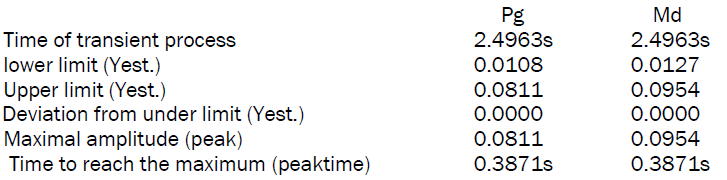
Research on simulator for other variants of tuning with the regulator shows that these are no better quality indicators than these because the whole action diapason is studied. In the static system there is an established error. The time of transient process – 2s can influence the quality of sustaining the rotation speed of GD and frequency of alternative current in the electric circuit. The shaft generator is linked strongly with the shaft of GD. That is why any action on perturbations system can negatively act on functioning conditions of the ship power electric station.
The specificity of representing the system dynamics in the form of transfer functions, equations in state space, in the model with zeros and poles, frequency characteristics and others, defines modeling means, synthesis and time regulating methods.
For improvement of dynamic properties of the system, we use the PID-regulator.
We note that in the control tools of MATLAB medium we can use the pid function. Function syntax:
C= pid(Kp,Ki,Kd,Tf)
Where Tf – time constant of the aperiodic element filter. The transfer function of pid-regulator model with parallel structure is:
 eq10
eq10
While choosing the tune parameters, we remind that the increase of Kp reduces the error in established regime but also reduces the stability margin on phase and amplitude, that is why some oscillations can occur. The introduction of integral coefficient Ki favours the reduction up to zero of static error in established regime due to the increase of transfer coefficient in low frequencies with reduction of phase stability margin. The increase of differential component kd also increases the transfer coefficient in high frequencies. As a result the aspect of transient process is ameliorated. The choice of Tf limits the action of high frequency noise on control system.If we return to the system on figure 1, and transfer functions (eq3 – eq5), we have the regulator as the block C(s). While studying the properties of the system, we considered Kp=1, Ki=0, Kd=0. This situation has excluded the regulator influence on the tune parameters. Let us study the possible improvement of quality tuning by the choice of PID– regulator parameters.
Let us first consider Kp=20. We have damped oscillations regime. Modeling is done with file sah794.m. Next we consider Ki=0.3 and Kd=1.2 and the transient processes are improved (figure 3). With the operator stepinfo (ω,t) to evaluate the indicators of transient processes in the model represented on upper graphic (figure 3), we have the following:
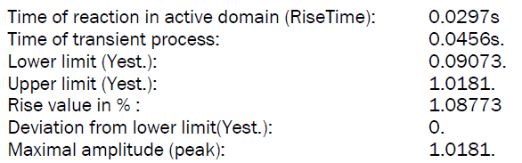

Figure 3: Representation of transient processes in the system with PID – regulator
We obtain the transfer functions of the closed – loop system with PID – regulator.
 eq11
eq11
 eq12
eq12
 eq13
eq13
The proper values of these expressions are:
λ1 = – 62.8704; λ2 = –175651; λ3 = –1.4394; λ4= –0.0150
In the interactive regime of MATLAB, we got a case similar to the one on eq11 – eq13, with the following values of coefficients: Kp=16.4837, Ki = 12.2345 and Kd = 0.72045. For modelling we used the pidtool function.
Finally, let us study the reaction of the system with PID – regulator on simultaneous actions of perturbations Md and Pg. For that purpose we consider rectangular form signal for the shaft generator and complex form signal for the torque. On figure 4, we represent the rotation speed ω(t) of diesel shaft (upper part of the figure), depending on input signals r(t), Md(t), Pg(t) represented on the lower part.

Figure 4: Rotation speed of diesel shaft on actions r(t)=1, Md(t), Pg (t)
From the graphics, it is proven that quality indicators of the system with PID - regulator are better than those in the static system. We have a good stability of the rotation speed of shaft generator and consequently generation of electrical energy with good quality in the ship network. Modelling with the use of MATLAB tools allows us to get simple precise solutions, to reduce the time of parametric optimisation and enables quantitative evaluation for decisions made. The modelling results can be confirmed on a simulator by introducing numerical parameters from a control center and getting results on a screen. The role of modelling while studying complex ship technical equipment and the improvement of exploitation level is very crucial.
Through an example of parametric tuning in this paper, we have shown that simulators can improve the decision making in control systems.