Research & Reviews: Journal of Ecology and Environmental Sciences
ISSN: 2347-7830
ISSN: 2347-7830
Arooj Bashir*, Rafia Saqib
Department of Economics, COMSATS University Islamabad, Islamabad, Pakistan
Received: 28-Dec-2023, Manuscript No. JEAES-23-123884; Editor assigned: 30-Dec-2023, Pre QC No. JEAES-23-123884 (PQ); Reviewed: 13-Jan-2024, QC No. JEAES-23-123884; Revised: 22-Jan-2025, Manuscript No. JEAES-23-123884 (R); Published: 29-Jan-2025, DOI: 10.4172/2347-7830.13.1.001
Citation: Bashir A, et al. Recent The Dynamics of Greenhouse Gas Emissions, Renewable Energy Consumption, and Economic Growth: Evidence from South Asian. RR J Ecol Environ Sci. 2025;13:001.
Copyright: © 2025 Bashir A, et al. This is an open-access article distributed under the terms of the Creative Commons Attribution License, which permits unrestricted use, distribution and reproduction in any medium, provided the original author and source are credited.
Visit for more related articles at Research & Reviews: Journal of Ecology and Environmental Sciences
Global warming and climate change, escalated by Greenhouse Gas (GHGs) emissions wreak a massive threat to human life and environment. Consequently, reducing environmental degradation is a prime global concern for sustainable development. The main purpose of current study is to explore a relationship between GHG proxies by CO2 emission, N2O emission, and CH4 emissions along with economic growth, renewable energy consumption, trade openness, and total natural resource rent for a panel of six selected South Asian countries. By using annual data from 1990-2020, and relevant methods for examining data properties, this study used panel ARDL methodology to determine a long-run and short-run relationship between selected variables. The panel results reveal the positive and significant impact of GDP on all three proxies of GHG emissions. Whereas, renewable energy has negative and significant impact on CO2 and N2O emissions. This study provides a comprehensive analysis of the determinants of renewable energy for South Asian countries. Furthermore, the empirical outcomes of current study delivers an imperative inference for policy-makers and highlight the role of renewable energy consumption in mitigating climate change in South Asian countries.
Environment; Renewable energy consumption; CO2; N2O
Human presence and economic activities cause global environmental fluctuations. The continuing growth of the global economy is a threat to the environment as outcome of amassed use of gasolines. Damages to environment and high energy consumption pays a major threat to the natural resources of the world. The industrial revolution caused climate change. Agriculture and industry have a significant impact on climate change, mainly as a result of the emissions of greenhouse gases and other pollutants. For its energy, the industry is highly dependent on fossil fuels, which means that large extents of CO2 end up in atmosphere. That’s main reason for the reinforced greenhouse effect. Although the emission of carbon dioxide has decreased, the greenhouse gas concentrations have increased, to 409.8 parts per million in 2019, the highest level in 800,000 years. The OECD report shows that South Korea is one of the countries with the worst air pollution and is expected to have the biggest rise in 2060. The annual health insurance report from South Korea shows that 19.5% of disease outbreaks are due to respiratory disorders caused by air pollution. Changes in climate sources over time and space also stimulate innovation in agricultural technology. It has been an important part of agricultural development. N2O is a by-product of agricultural and industrial processes and is important because of its considerable contribution to global warming. The emission of laughing gas is closely linked to agricultural practices, which raises questions about its impact on food security and economic growth. The globalization of trade has consequences for the emission of laughing gas through freight transport and the cross-border movements of emission-intensive industries. Understanding the relationship between global trading patterns and the emission of nitrogen oxide is crucial for developing international strategies for emission reduction [1]. Changes in agricultural productivity, influenced by climate-related factors related to N2O emissions, can have domino effects on local and global economies.
Agricultural sector in particular the nitrogen art and livestock farming activities, remains an important source of the emission of nitrogen dioxide. Reducing laughing gas emissions requires a comprehensive policy framework. Policy interventions aimed at promoting sustainable agricultural practices, technological innovation and emission reduction strategies play a crucial role in tackling the ecological and economic challenges associated with the emission of nitrogen oxide. Mitigation strategies for these emissions are crucial to achieve sustainable development. The consequences for the environment of laughing emissions extend to the economy. The emission of greenhouse gases will have an impact on climate change. That can also be influence various economic sectors, including agriculture, energy and infrastructure.
Both natural resources and human and industrial capital contribute considerably to the economic growth of countries. In developing countries, of course, capital complements or replaces the capital made by humans in production, thereby guaranteeing the sustainability of the environment. Governments can use income from resources and taxes to finance infrastructure projects and the formation of human capital, which promotes economic growth, especially in developing countries with capital scarcity, where income from natural resources supplement the limited budget capacity to spend human capital [2]. The use of natural resources to obtain economic benefits is reflected in the total yield of natural resources. Balancing the extraction and preservation of resources is crucial for a long-term sustainable development found negative effects.
However, measuring the damage caused by human activities to the environment is not the only way to measure the sustainability of the environment. It is rather interesting to assess, synthesize and clarify what the proceeds of bio capacity have to offer. The relationship between yields from resources and economic growth entails complex dynamics that influences both advanced and development economies. Current scientific literature on the importance of natural resources in relation to GDP still has to offer a comprehensive analysis of the complex dynamics that arise during digitization. There is still a lack of insight into the impact of renovation of economies mainly depend upon natural resources. According to Sharma and Paramati, resource capital is a benchmark for the resources of resources of a country or its natural resources. Leasing natural resources is an alternative to the consumption of resources. The extraction and use of minerals and natural gas contributes considerably to the natural gas profits in emerging economies such as China, but there is no empirical evidence that the real relationship between North Korea and GDP supports.
International trade plays a key role in shaping global environmental results. Although trade can decentralize pollution intensive industries, it also raises questions about environmental justice and sustainability. Trade policy and trade agreements can influence the quality of the environment and on the balance between economic growth and environmental protection. Although trading liberalization policy has stimulated economic growth, the potential has been examined Negative consequences for the environment. Critics claim that an unbridled focus on economic growth through trade could lead to greater extraction of resources, deforestation and pollution. The consequences for the environment of the liberalization of trade are a key factor in discussions about sustainable development. Green trade concepts that give priority to the exchange of ecologically sustainable products and services are becoming increasingly important. The literature on green trade emphasizes the need to develop policy that encourages environmentally friendly production and to investigate the potential of trade to make a positive contribution to ecological sustainability and economic growth. Encouraging sustainable consumption patterns through trade policy and trade agreements is seen as a strategy to combine economic growth with ecological sustainability.
The persistent increase in global warming and its negative consequences for climate increase the urgency of making the global system carbon -free. The growth of renewable energy is extremely important and efficient. It is also a time-saving step towards achieving decarbonization objectives. In the early 1990's, the public awareness of the problems with environmental pollution increased. Renewable energy, on the other hand, is constantly being renewed and has less negative impact on the environment. It reduces carbon dioxide emissions, protects the environment, reduces dependence on foreign resources and increases employment. Research shows that contrary bond amid deterioration of environment and monetary progress, influenced by economic growth, structure, energy dependence and efficiency [3]. The global demand for energy will grow by 30% between 2016 and 2040. This is comparable to the current growth of global demand in China and other parts of India. To tackle these problems, sustainable practices are needed with the emphasis on renewable energy to reduce nitrogen dioxide emissions and to combat climate change. The balance between economic development and the environment is crucial for a sustainable future.
The present study focusses on the selected sample of South Asian countries because the economically emerging South Asian countries are noticed as the most vulnerable region due to the climate related changes globally. The present study contributes to the prior literature in the following strands. First, unlike previous studies on the relationship among CO2 emission and economic growth, this study has employed CO2, N2O, and NH4 as proxies of environmental degradation to find out the dynamics between the GHGs, economic growth and renewable energy consumption. To the best of our knowledge, this is the first study that includes natural resource rent in the relationship among environment and income for South Asian countries. Hence, the motivation of the current research is to explore the relationship in GHGs and role of economic growth, renewable energy consumption, trade openness, and natural resource rent in the selected South Asian.
The rest of this paper is organized as follows. The ‘‘Literature Review’’ section states the previous panel theory and research of GHG emissions impact factor nexus. The ‘‘Data and Methodology’’ section briefly discusses the data, model specification and panel techniques. Then, ‘‘Results and Discussion’’ show the empirical findings and detailed discussion. Finally, in ‘‘Conclusion’’ section we conclude this study and provide some policy implications.
Environmental degradation was formerly mostly linked to CO2 emissions from industrialized nations. But because of their rapid industrialization and economic expansion, emerging nations have gained a lot of attention recently. Nitrogen dioxide, a major air pollutant primarily emitted by combustion processes, industrial activities, and transportation, has far-reaching environmental and human health consequences. It plays a significant role in climate change because NO2 contributes to the formation of tropospheric ozone and fine particulate matter, both of which influence regional and global climate patterns. The complex interplay of Nitrogen Dioxide (NO2), climate change, and economic growth highlights the multifaceted challenges confronting our global community. Numerous studies explore the role of innovation in advancing renewable energy technologies. Innovations in solar, wind, and other clean energy sources are crucial for reducing reliance on fossil fuels and mitigating climate change.
Herranz, et al. investigated the relationship among economic growth and environmental pollution in 17 OECD states from 1990 to 2012. Founded that an N-shaped relationship exists between income and environmental degradation. Environmental pollution. Influence. Increase in greenhouse gas emissions. The relationship between economic growth and environmental sustainability is complex. Potential for “green growth” continues for debate.
Scholars argue for decoupling economic growth from environmental degradation through technological innovation, policy interventions, and sustainable practices. Researchers believe that economic growth should be disconnected from the damage to the environment through technological innovation, policy intervention and sustainable practices. Sinha investigated the relationship between nitrogen dioxide, economic growth and inequality in energy intensity in 139 cities in India from 2001 to 2013 [4]. The results prove the feedback hypothesis and the existence of Kuznet's curve for both pollutants. These results are crucial for policy makers to develop a sustainable economic policy. Degraeuwe investigated the driving forces behind the emissions of nitrogen dioxide in Belgium [5]. Their research showed that, although Belgium has comparable characteristics of stable growth in urbanization, there are significant differences between countries in terms of CO2 emissions per head of the population, the energy mix and energy intensity. Hilboll, et al. significant economic growth in India [6]. Satellite pay detection makes it possible to monitor air pollution. From 2003 to 2012, pollution due to nitrogen dioxide was closely linked to economic growth, with an annual growth rate of no less than 4.4%. But since 2012, pollution by nitrogen dioxide has stabilized or has a downward trend. Regional sources of pollution, such as steel smiles and the cement industry, the air quality deteriorate. Cui, et al. calculated the link concerning economic activities and air pollution [7]. Discovered that policy measures resulted in a significant reduction in pollution due to nitrogen dioxide. They also noted that economic events such as the 2008 financial crisis, COVID-19 and armed conflicts also affect the air quality.
Ploeg FV investigates the potential advantages and disadvantages of natural resources, with the argument that they can be a blessing or a curse [8]. Hypotheses suggest that the hawse can lead to raw materials to the disposalization, weak growth and corruption, especially in unstable countries with weak institutions and underdeveloped financial systems. Akpan GE and Chuku C [9]. assess that greater financing and participation in education shifts the comparative benefit from the production of natural resources to production and services. Venables AJ discuss the challenges and reasons for disappointing results [10]. Development economies strive to use the wealth of natural resources to improve economic performance. This includes private investments, the financial system, sensible expenses and policy. The experiences are mixed, with some successes in countries such as Botswana and Malaysia. Mohamed ESE analysis of the institutional impact of Sudan on the abundance of resources and the long-term balance relationship between the yields of resources, human development and economic growth [11]. Economic growth is positively influenced by rental prices and developmental spending, while life expectancy negatively influences growth. Managing income from natural resources promotes sustainable growth. Lou G investigated the economic output of China from 1987 to 2022, which showed that trade and energy efficiency make an important contribution, but hinder further development [12]. Natural capitals have short -term benefits that become negative over time, which leads to China's resource curse.
Copeland investigates the benefits of prosperity improving policy reforms in small open economies that suffer from trade disruptions and pollution [13]. He compares taxes, quotas and mixed systems and comes to the conclusion that the welfare benefits of reforms of pollution policy are greater in economies with international factor mobility. Antweiler, et al. investigated the impact of international raw material markets on the concentrations of pollution [14]. He suggested a theoretical model that divided the effects of trade into scale effects, technology effects and composition effects. As a result, international trade reduces pollution concentrations when the composition of national production changes. Free trade is generally good for the environment. Yunfeng Y and Laike Y discovered that world trade has a significant impact on the environment, since consumers transfer pollution to other countries [15]. From 1997 to 2007, the emissions of carbon dioxide by Foreign Trade of China was responsible for 10.03% to 26.54% of annual emissions, while imports only 4.40% to 9.05% were responsible for. Dale, Jones and Olkin are investigating the impact of historical temperature fluctuations on economic results. The results show that rising temperatures considerably reduce economic growth in poor countries, which can influence the growth rates that go beyond the production level. The findings emphasize the potential negative consequences of rising temperatures for agriculture, industry and political stability.
Ali, et al. investigated the relationship between trade, eco-innovation and the consumption of renewable energy in the top 10 of carbon pruning countries. The results show cross-sectional dependence and long-term balancing relationships, which are important factors in explaining consumption-based and regional carbon emissions. Bamati N, and Raoofi A investigates the factors that drive the creation of renewable energy in industrialized and emerging countries, with the help of technical, economic and ecological considerations [16]. The results show that the production of renewable energy is influenced by exports from industrialized countries. Although the impact of oil prices is smaller. Renewable energy has a positive impact on GDP per head of the population. Carbon dioxide is considerably different. Sarkodie, et al. studied the impact of income, renewable energy, direct foreign investments and administration on the emissions of greenhouse gases in 47 countries south of the Sahara between 1990 and 2017 [17]. They discovered that by increasing the consumption of renewable Energy the emissions fell. Increases in income, administration and consumption of renewable energy worsen climate change. Research shows that the consumption of renewable energy reduces the impact of climate change. This speeds up the transition from fossil fuels to energy efficiency by disconnecting them from economic growth. Afroz R and Muhibbullah M explored that national renewable energy and energy consumption have an asymmetrical impact on economic growth, in which consumption leads to increased CO2 emissions from unconventional energy sources [18]. Reduction of renewable energy can accelerate economic growth, while reducing renewable energy can lead to an economic recession. The study proposes measures to reduce the dependence on renewable energy sources for natural energy consumption. Abbas, et al. measured that there are long-term symmetrical and asymmetrical relationships in which market regulation plays an important role [19]. This literature overview paves the way for an extensive research into the relationship between the emissions of N2O, renewable energy, trade, the total yields of natural resources and economic growth. By synthesizing existing knowledge, this study wants to provide valuable insights into current sustainability discussions.
Data description
To explore the determinants of environmental degradation (CO2, N2O, CH4) and scrutinize the role of Renewable Energy Consumption (REC) this present research relies a panel data set from 1990-2020 of selected Asian countries including Bangladesh, Bhutan, India, Nepal, Pakistan, and Sri Lanka retrieved from World Development Indicator (WDI). The other South Asian countries (Maldives and Bangladesh) are excluded from the dataset due to the non-availability of the data. The variables included in the study are Carbon Dioxide (CO2) emission, Nitrous Oxide (N2O) emission, Methene (CH4) emission, per capita GDP (Y), Renewable Energy Consumption (REC), Trade (TR), and Total Natural Resource (TNR) rent. An explanatory explanation of the related variables and dataset used for the econometric analysis is presented in Table 1. To find out the long-run relationship among the selected variables, we transformed the model into natural logs. Normalization of data into natural log linear model can generate efficient results, mitigates dynamic distortion, and induce the stationarity. The log-linear model is expressed as:
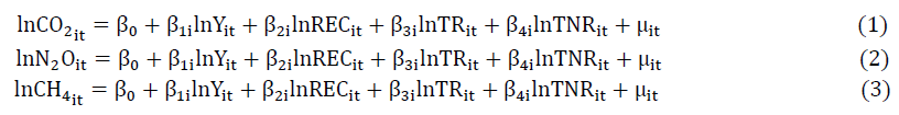
Where, (i=1, ……., 6 countries) and (t=1990, ……., 202) represents the cross section and time dimension respectively; β1, β2, β3, β4 indicates the undermined coefficients. Symbol ln indicates that the variables are in logarithm form.
Methodology
In current study, we used the sbalanced panel data set. Existence of Cross-sectional Dependence (CD) is the one of the assumption of panel data, which may generate biased and unreliable results. Before panel cointegration test, it is mandatory to perform cross-sectional independence and homogeneity test. It is assumed that to determine the cross-sectional dependence Breusch and Pagan, Pesaran, and pesaran were used. The test statistics is calculated as in Equation 2 in the study proposed by Breusch and Pagan:
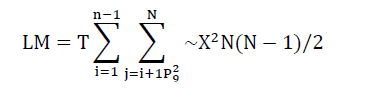
The LM test is valid in cases where the dimension of N is small and the dimension of T is large. The test statistics is developed by Pesaran is found in Equation 2.
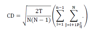
Under the null hypothesis, when T is sufficiently large, the limit of the CD→ (0, 1) function is N→∞. In this case where T→∞ and the N→∞ for large panels, Pesaran, et al. suggest a corrected version of LM test. The corrected LM test is expressed as follows:
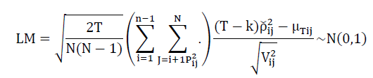
Here, k is the number of regressors, and μTij and Vij 2 are the mean and variance respectively of (T-k)ρ�?ij 2 is developed by Pesaran, et al.
In horizontal section dependence tests, the hypothesis is:
H0: “There is no dependence between sections.”
H1: “There is dependence between sections.”
According to the test results, if H0 hypothesis cannot be rejected, the analysis with first generation panel unit root test. However, if the H0 hypothesis is rejected, it will be corrected to continue the analysis with second generation panel unit root tests.
The next step is to check the stationary properties of the selected variables to find out the co-integration order for the presence of long-run relationship. In literature, there are many types of unit root test are available for confirming the co-integration. In this study, we used the CIPS unit root test presented by Pesaran. This unit root test generates reliable results in presence of CD as compared to traditional methods. The panel IPS test is more powerful as compared to other. The CIPS unit root is presented as:
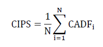
Where CADFi is a cross-sectional augmented dickey fuller statistic.
Pedroni cointegration is the widely used co-integration test has proposed seven co-integrations in its two types of tests. One is called within dimension approach and other is between dimension approaches. In within dimension four statistics (panel v statistics, panel PP-statistics, panel ADF t-statistics and panel rho-statistics) are included. The autoregressive coefficients of the residuals are pooled by these four statistics. Other approach which is called between dimension has three statistics (Group rho-Statistics, Group PP-Statistics, Group ADF-Statistics) are derived by taking average of all individual autoregressive coefficient. These autoregressive coefficients are linked with individual unit roots of residuals of each cross section in panel.
To analyze the short-run and long-run relationship among variables, we implemented the panel ARDL proposed by Pesaran:

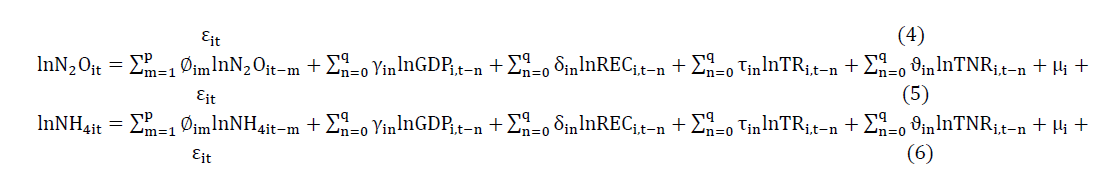
Where γin, δin, τin, ϑin are 1xK vector of coefficients of the regressors, ∅im presented the scalers of coefficients of lagged dependent variables. Equation 4-6 is reparametrized for both short-run and long run dynamics and coefficients, as follows:
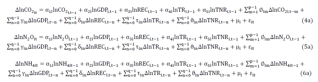
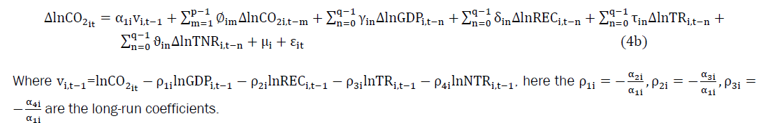
The error correction form is presented as follows:
The last step is to analyze the causality direction among the selected variables. In this regard, we used D-H causality test proposed by Khoshnevis Yazdi and Golestani Dariani as it is an befitting approach for the directional causality and presents more advantages compares to the tradition Granger causality test [20]. DH causality test presents two spheres of heterogeneity, known as heterogeneity of the regression model and heterogeneity of the causal relationship. The hypothesis of DH test
Where Wi,T represents the values of individual Wald statistics for cross-sectional units.
| Variable | Symbol | Metrics and descriptions | Unit |
| Carbon dioxide | CO2 | Carbon dioxide emissions are those stemming from the burning of fossil fuels and the manufacture of cement. They include carbon dioxide produced during consumption of solid, liquid, and gas fuels and gas flaring. | CO2 emissions (kt) |
| Nitrous oxide | N2O | Nitrous oxide emissions are emissions from agricultural biomass burning, industrial activities, and livestock management. | Thousand metric tons of CO2 equivalent |
| Methene | CH4 | Methane emissions are those stemming from human activities such as agriculture and from industrial methane production. | kt of CO2 equivalent |
| Economic growth | GDP | Gross domestic product of each country | Constant 2017 international $ |
| Renewable Energy consumption | REC | Renewable energy consumption is the share of renewable energy in total final energy consumption. | Renewable energy consumption (% of total final energy consumption) |
| Trade | TR | Trade is the sum of exports and imports of goods and services measured as a share of gross domestic product. | Percentage of GDP |
| Natural resource rent | TNR | Total natural resources rents are the sum of oil rents, natural gas rents, coal rents (hard and soft), mineral rents, and forest rents. | Total natural resources rents (% of GDP) |
Table 1. Variable symbols, names, and unit.
Cross-sectional Dependence (CD)
The empirical investigation of the present study begins with the Cross-sectional Dependence (CD) estimations. South Asian countries such as Bangladesh, Bhutan, India, Nepal, Pakistan, and Sri-Lanka are being caused from the CD, cross-country heterogeneity, and effect of trans-border pollutants. Due to the different characteristics of the countries, the present study performed the CD test and CD tests. The results of both CD test are presented in Table 2, which denies the null hypothesis of no Cross-sectional Dependence (CD) at 1% level of significance. It is concluded that there is strong evidence of the presence of CD among the variables such as lnN2O, lnGDP, lnREC, lnTR, and lnTRN in case of South Asian countries.
|
Breusch-Pagan LM |
Pesaran CD |
|||
|
Variable |
Statistics |
Prob. |
Statistics |
Prob. |
|
lnCO2 |
388.7786 |
0.000*** |
19.70041 |
0.000*** |
|
lnN2O |
247.0134 |
0.000*** |
9.945918 |
0.000*** |
|
lnCH4 |
311.2521 |
0.000*** |
1.081643 |
0.000*** |
|
lnGDP |
454.2975 |
0.000*** |
21.31347 |
0.000*** |
|
lREC |
370.029 |
0.000*** |
19.19612 |
0.000*** |
|
lnTR |
87.96255 |
0.000*** |
2.773328 |
0.000*** |
|
lnTNR |
140.9273 |
0.000*** |
6.908171 |
0.000*** |
|
Note: ***: Shows level of significance at 1%. |
||||
Table 2. The presence of CD among the variables such as lnN2O, lnGDP, lnREC, lnTR, and lnTRN in case of South Asian
Panel unit root
The presence of CD in the variables leads to biased and unreliable results due to the different characteristics of the countries. To handle the ambiguity of CD in the sample data, we performed the second generation unit root test to see that the variables should not be I (2); otherwise, the results will be spurious. The results of panel unit root test for each variable are presented in Table 3. The findings of unit root test shows that all variables except lnCO2, lnTR could not be rejected as null. In contrast, the null hypothesis for all variables is rejected at 1%, and 5% significance level when tested series are in 1st difference. Therefore, it is concluded that all variables are integrated of the order one I (1). The mixed order of integration provides suitability of panel ARDL methodology to find out the short and long coefficients.
| Variables | Level | 1st Difference |
| lnCO2 | -2.83666* | -2.86490** |
| lnN2O | -2.53736 | -4.32679*** |
| lnCH4 | -1.79316 | -5.22741*** |
| lnGDP | -1.97703 | -3.73074*** |
| lnREC | -2.14031 | -2.89777** |
| lnTR | -2.75740* | -4.43316*** |
| lnTNR | -2.04226 | -3.05196** |
| Note: *, **, ***: Indicates the level of significance at 1, 5, and 10 percent respectively | ||
Table 3. Findings of CIPS unit root test analysis.
Panel co-integration test
The next step after estimating the pre specification of panel co-integration test is applying the Pedroni co-integration test. The Findings of panel co-integration of model 1 is presented in Table 4. The results illustrated that a set of four statistics are significant at 1% and 5% level of significance. As the total numbers of statistics are eleven in number out of those four are significant, so null hypothesis cannot be rejected. So, we conclude that there is no co-integration among the variables. The results for CH4, presented in Table 2 is similar to the findings of these.
| Tests | Statistics | Prob. | W. statistics | Prob. | |
| Panel v-statistics | 0.548046 | 0.2819 | -2.23166 | 0.9872 |
|
| Panel rho-statistics | 0.765815 | 0.7781 | 1.932717 | 0.9734 |
|
| Panel PP-statistics | -0.88514 | 0.188 | -1.59998 | 0.0548* |
|
| Panel ADF-statistics | -0.72128 | 0.2354 | -3.27972 | 0.000*** |
|
| Group rho-statistics | 1.61598 | 0.947 |
|
||
| Group PP-statistics | -2.96936 | 0.0015*** |
|
||
| Group ADF-statistics | -2.47597 | 0.0066*** |
|
||
| Note: *, **, *** Indicates the level of significance at 1, 5 and 10 percent respectively. |
|
||||
Table 4. Findings of pedroni co-integration test analysis for model 1 (CO2).
Whereas, the results of N2O presented in Tables 5 and 6, illustrated that a set of seven statistics are significant at 1% level of significance. As the total numbers of statistics are eleven in number out of those seven i.e., majority is having probabilities that are less than 5%, so null hypothesis can be rejected. So, we conclude that there is co-integration among the variables. The estimation results indicate that economic growth, renewable energy consumption, trade, and natural resource rent are all connected to N2O emission in long-run equilibrium over the period considered.
| Tests | Statistics | Prob. | W. statistics | Prob. |
| Panel v-statistics | 4.726241 | 0.0000*** | 1.959642 | 0.025** |
| Panel rho-statistics | -0.05388 | 0.4785 | 0.926223 | 0.8228 |
| Panel PP-statistics | -4.14919 | 0.0000*** | -2.34003 | 0.0096*** |
| Panel ADF-statistics | -3.88637 | 0.0001*** | -1.04377 | 0.1483 |
| Group rho-statistics | 1.848639 | 0.9677 | ||
| Group PP-statistics | -2.73513 | 0.0031*** | ||
| Group ADF-statistics | -1.28777 | 0.0989* | ||
| Note: *, **, *** Indicates the level of significance at 1, 5 and 10 percent respectively. | ||||
Table 5. Findings of pedroni co-integration test analysis for model 2 (N2O).
| Tests | Statistics | Prob. | W. statistics | Prob. |
| Panel v-statistics | -0.35137 | 0.6373 | 0.575984 | 0.2823 |
| Panel rho-statistics | 2.822115 | 0.9976 | 1.704993 | 0.9559 |
| Panel PP-statistics | 2.940324 | 0.9984 | -0.86105 | 0.9416 |
| Panel ADF-statistics | -1.41215 | 0.0790* | -4.18185 | 0.0000*** |
| Group rho-statistics | 2.524227 | 0.9942 | ||
| Group PP-statistics | -2.29535 | 0.0109** | ||
| Group ADF-statistics | -3.14319 | 0.0000*** | ||
| Note: *, **, *** Indicates the level of significance at 1, 5 and 10 percent respectively. | ||||
Table 6. Findings of pedroni co-integration test analysis for model 3 (NH4).
Panel ARDL test
The present study aims to investigate the relationship between GHGs, economic growth and renewable energy consumption along with some the explanatory variables. Therefore, we applied the panel ARDL model presented by Pesaran. Panel ARDL model is used to explain the short-run and long-run dynamics of the selected variables. The ARDL results for model 1 lnCO2 is presented in Table 7. In the long run, the coefficient of lnGDP was found to have a positively significant effect on carbon emission. This shows that rise in economic activities in panel of South Asian countries will result in rise in carbon dioxide emission. This finding is in-line with the findings of Yusuf. The coefficient of lnREC is negative and significant impact on carbon dioxide emission, showing that increase in usage of renewable energy consumption is associated with decrease in emission. Trade has positive and significant effect on CO2 emission, as increase in trade will cause an increase in emissions. Whereas, the coefficient of lnTNR is negative but insignificant. However, in short run, we only found a negative and significant impact of lnREC on CO2 emission. The error correction term show that the speed of adjustment back towards the equilibrium is corrected by 0.01% in South Asian country’s panel in each year.
| Variables | Long run | Short run |
| lnGDP | 0.526657 (0.0012)*** | 0.09334 (0.7922) |
| lnREC | -1.204432 (0.0000)*** | -3.004911 (0.0294)** |
| lnTR | 0.07076 (0.0370)** | -0.042138 (0.1256) |
| lnTNR | -0.01226 (0.4883) | 0.022099 (0.2788) |
| ECT | -2.287605 (0.0144)** | |
| Note: *, **, *** Indicates the level of significance at 1, 5 and 10 percent respectively. | ||
Table 7. Panel ARDL estimates of model 1 (CO2).
The panel ARDL estimations of model 2 presented in Table 8. The results shows that lnGDP, lnREC, lnTR are a significant and positive contribution to N2O emission in considered panel. It means that economic activities in South Asian region deteriorated the environmental quality. Economic growth in the panel increased the N2O emission. It is also observed that lREC has a significant and positive contribution to N2O emission. This suggests that 1% increasing the consumption of renewable energy consumption leads to increase N2O emission by 1.5%. Our results are in-line with the results of. Concerning the negative and significant coefficient of lnTNR, indicates that lnTNR diminishes the N2O emission. Converting to traditional technologies initiating exploitation of natural resources to advanced technologies that assimilate recycling, value-addition, reprocessing, and artificial resources that replace natural resources will lead to better environmental. Moreover, the significant terms confirm the long-run relationship among selected variables. The error correction term show that the speed of adjustment back towards the equilibrium is corrected by 40% in South Asian country’s panel in each year. For the short-run analysis, we found that lnREC, and lnTR has a negative and significant impact on N2O emission, while lnTNR has a positive and significant impact on N2O emission. However, we did not find any short run relationship among lnGDP and lnN2O emission.
|
|||||||||||||||||||||
Table 8. Findings of panel ARDL test of N2O.
Table 9 presented the panel ARDL estimations of CH4. According to the results, lnGDP increases the methene emission significantly at 1% level of significance. The coefficient of lnREC is negative but has insignificant impact on methane emissions. The insignificant impact of lnREC accredited to the less usage of renewable energy on production, services, and industrial sectors. Concerning to the results of lnTR, it has positive and significant effect on the environmental degradation. It is concluded that trade activities in the South Asian economies has damaged the environmental conditions. It is estimated that lnTNR has positive and significant effect on methane emission in panel of south Asian countries.
| Variables | Long run | Short run |
| lnGDP | 0.150425 (0.0156)*** | 0.014169 (0.6656) |
| lnREC | -0.029362 (0.5928) | -0.077260 (0.5909) |
| lnTR | 0.08316 (0.0000)*** | -0.022239 (0.4006) |
| lnTNR | 0.025298 (0.0003)*** | 0.014837 (0.2797) |
| ECT | -0.366987 (0.0056)*** | |
| Note: Lag length (2,2,2,2) (The selection of optimal lag length is based on AIC) *,**,*** shows 10%, 5%, and 1% level of significance. | ||
Table 9. Panel ARDL estimates of CH4 model.
Pairwise Dumitrescu Hurlin (DH) panel causality
The results of panel ARDL model indicates the short-run and long-run relationship among a set of variables. Nevertheless, it does not determine the causality direction among the variables. Therefore, Table 10 summarizes the causality direction of the selected variables in south Asia for CO2 emission. The results indicate that there are uni-directional causalities are running from lnGDP to lnCO2, lnREC to CO2, lnTR to lnGDP, lnREC to lnTNR, and lnTR to lnTNR. Whereas, bi-directionaly causality running between lnCO2 and lnTNR, lnGDP and lnREC, lnGDP and lnTNR. However, no causality direction found between lnTR and lnCO2, and lnTR and lnREC.
| Null hypothesis | W-stat. | Zbar-stat. | Prob. | Results | |
| lnGDP does not homogeneously cause lnCO2 | 4.62648 | 2.50545 | 0.0122 | Reject H0 | lnGDP→lnCO2 |
| lnCO2 does not homogeneously cause lnGDP | 3.66419 | 1.51923 | 0.1287 | Accept H0 | |
| lnREC does not homogeneously cause lnCO2 | 3.94673 | 1.8088 | 7.05E-02 | Reject H0 | lnREC→ln CO2 |
| lnCO2 does not homogeneously cause lnREC | 3.53952 | 1.39147 | 0.1641 | Accept H0 | |
| lnTR does not homogeneously cause lnCO2 | 3.48284 | 1.33338 | 1.82E-01 | Accept H0 | - |
| lnCO2 does not homogeneously cause lnTR | 3.17099 | 1.01377 | 0.3107 | Accept H0 | |
| lnTNR does not homogeneously cause lnCO2 | 4.46957 | 2.34463 | 0.019 | Reject H0 | lnCO2↔lnTNR |
| lnCO2 does not homogeneously cause lnTNR | 11.8565 | 9.9152 | 0 | Reject H0 | |
| lnREC does not homogeneously cause lnGDP | 6.79366 | 4.72651 | 2.00E-06 | Reject H0 | lnGDP↔lnREC |
| lnGDP does not homogeneously cause lnREC | 6.7124 | 4.64323 | 3.00E-06 | Reject H0 | |
| lnTR does not homogeneously cause lnGDP | 3.08682 | 0.9275 | 0.3537 | Accept H0 | lnTR→lnGDP |
| lnGDP does not homogeneously cause lnTR | 4.85469 | 2.73933 | 0.0062 | Reject H0 | |
| lnTNR does not homogeneously cause lnGDP | 3.97361 | 1.83635 | 0.0663 | Reject H0 | lnGDP↔lnTNR |
| lnGDP does not homogeneously cause lnTNR | 6.50846 | 4.43422 | 9.00E-06 | Reject H0 | |
| lnTR does not homogeneously cause lnREC | 3.50053 | 1.3515 | 0.1765 | Accept H0 | - |
| lnREC does not homogeneously cause lnTR | 3.39207 | 1.24035 | 0.2148 | Accept H0 | |
| lnTNR does not homogeneously cause lnREC | 2.81081 | 0.64464 | 0.5192 | Accept H0 | lnREC→lnTNR |
| lnREC does not homogeneously cause lnTNR | 10.9645 | 9.00108 | 0 | Reject H0 | |
| lnTNR does not homogeneously cause lnTR | 4.57854 | 2.45632 | 0.014 | Reject H0 | lnTNR→lnTR |
| lnTR does not homogeneously cause lnTNR | 1.08738 | -1.12165 | 0.262 | Accept H0 |
Table 10. Pairwise Dumitrescu Hurlin (DH) panel causality test for model 1 (CO2).
Table 11 presented the D-H causality estimation for N2O. From results, we found that one-way causality runs from lnGDP to lnREC, lnN2O to lnREC, lnN2O to lnTR, lnTNR to lnTR. Furthermore, we found a bi-directional causality between lnTR and lnGDP, lnTNR and lnGDP, lnTR and lnREC, lnTNR and lnREC. However, there is no causality relationship among lnTNR and lnN2O emission found in the estimations.
| Null hypothesis | W-stat. | Zbar-stat. | Prob. | Results | |
| lnGDP does not homogeneously cause lnN2O | 2.8504 | 2.67046 | 0.0076*** | Reject H0 | LGDP→LN2O |
| lnN2O does not homogeneously cause lnGDP | 1.82362 | 1.12167 | 0.262 | Accept H0 | |
| lnREC does not homogeneously cause lnN2O | 1.73749 | 0.99175 | 0.3213 | Accept H0 | LN2O→LREC |
| lnN2O does not homogeneously cause lnREC | 2.87505 | 2.70764 | 0.006*** | Reject H0 | |
| lnTR does not homogeneously cause lnN2O | 0.33697 | -1.12079 | 0.2624 | Accept H0 | LN2O→LTR |
| lnN2O does not homogeneously cause lnTR | 2.72825 | 2.48621 | 0.0129** | Reject H0 | |
| lnTNR does not homogeneously cause lnN2O | 1.46252 | 0.57698 | 0.564 | Accept H0 | - |
| lnN2O does not homogeneously cause lnTNR | 1.79818 | 1.0833 | 0.2787 | Accept H0 | |
| lnREC does not homogeneously cause lnGDP | 2.03164 | 1.43544 | 0.1512 | Accept H0 | LGDP→LREC |
| lnGDP does not homogeneously cause lnREC | 3.4639 | 3.59586 | 0.0003*** | Reject H0 | |
| lnTR does not homogeneously cause lnGDP | 4.25038 | 4.78218 | 0.000*** | Reject H0 | LTR↔LGDP |
| lnGDP does not homogeneously cause lnTR | 2.9925 | 2.8848 | 0.0039*** | Reject H0 | |
| lnTNR does not homogeneously cause lnGDP | 2.18819 | 1.67158 | 0.0946* | Reject H0 | LTNR↔LGDP |
| lnGDP does not homogeneously cause lnTNR | 2.93897 | 2.80406 | 0.005*** | Reject H0 | |
| lnTR does not homogeneously cause lnREC | 3.3947 | 3.49147 | 0.0005*** | Reject H0 | LTR↔LREC |
| lnREC does not homogeneously cause lnTR | 2.82843 | 2.63732 | 0.0084*** | Reject H0 | |
| lnTNR does not homogeneously cause lnREC | 3.06873 | 2.99979 | 0.0027*** | Reject H0 | LTNR↔LREC |
| lnREC does not homogeneously cause lnTNR | 9.21677 | 12.2734 | 0.000*** | Reject H0 | |
| lnTNR does not homogeneously cause lnTR | 2.59465 | 2.28468 | 0.0223** | Reject H0 | LTNR→LTR |
| lnTR does not homogeneously cause lnTNR | 0.67754 | -0.60707 | 0.5438 | Accept H0 | |
| Note: Lag length 1. | |||||
For CH4 the results are presented in Table 12. the estimated results indicates that one-way causality runs from ln NH4 to lnGDP, lnGDP to lnTR, lnTNR to lnGDP, lnREC to lnTNR, and lnTNR to lnTR. Besides, we found a bi-directional causality between lnREC and lnGDP.
| Null hypothesis | W-stat. | Zbar-stat. | Prob. | Results | |
| lnGDP does not homogeneously cause lnCH4 | 3.41052 | 1.25925 | 0.2079 | Accept H0 | lnCH4→lnGDP |
| lnCH4 does not homogeneously cause lnGDP | 4.18613 | 2.05414 | 0.04 | Reject H0 | |
| lnREC does not homogeneously cause lnCH4 | 3.44328 | 1.29283 | 0.1961 | Accept H0 | - |
| lnCH4 does not homogeneously cause lnREC | 3.66396 | 1.519 | 0.1288 | Accept H0 | |
| lnTR does not homogeneously cause lnCH4 | 3.09534 | 0.93623 | 0.3492 | Accept H0 | - |
| lnCH4 does not homogeneously cause lnTR | 2.82841 | 0.66267 | 0.5075 | Accept H0 | |
| lnTNR does not homogeneously cause lnCH4 | 2.18874 | 0.00709 | 0.9943 | Accept H0 | |
| lnCH4 does not homogeneously cause lnTNR | 2.26131 | 0.08147 | 0.9351 | Accept H0 | - |
| lnREC does not homogeneously cause lnGDP | 6.79366 | 4.72651 | 2.00E-06 | Reject H0 | |
| lnGDP does not homogeneously cause lnREC | 6.7124 | 4.64323 | 3.00E-06 | Reject H0 | lnREC↔lnGDP |
| lnTR does not homogeneously cause lnGDP | 3.08682 | 0.9275 | 0.3537 | Accept H0 | lnGDP→lnTR |
| lnGDP does not homogeneously cause lnTR | 4.85469 | 2.73933 | 0.0062 | Reject H0 | |
| lnTNR does not homogeneously cause lnGDP | 3.97361 | 1.83635 | 0.0663 | Reject H0 | lnTNR→lnGDP |
| lnGDP does not homogeneously cause lnTNR | 6.50846 | 4.43422 | 9.00E-06 | Reject H0 | |
| lnTR does not homogeneously cause lnREC | 3.50053 | 1.3515 | 0.1765 | Accept H0 | - |
| lnREC does not homogeneously cause lnTR | 3.39207 | 1.24035 | 0.2148 | Accept H0 | |
| lnTNR does not homogeneously cause lnREC | 2.81081 | 0.64464 | 0.5192 | Accept H0 | lnREC→lnTNR |
| lnREC does not homogeneously cause lnTNR | 10.9645 | 9.00108 | 0.0000 | Reject H0 | |
| lnTNR does not homogeneously cause lnTR | 4.57854 | 2.45632 | 0.014 | Reject H0 | lnTNR→lnTR |
| lnTR does not homogeneously cause lnTNR | 1.08738 | -1.12165 | 0.262 | Accept H0 |
Table 12. Pairwise Dumitrescu Hurlin (DH) panel causality test for model 3 (CH4).
The dynamics between emissions, growth, and energy is one of the most important topic for academia, researchers, and policy makers alike. In present research, we tried to carried out three different proxies of environmental degradation (i.e., CO2, N2O, CH4) to find out the relationship with economic growth (GDP), Renewable Energy Consumption (REC), Trade Openness (TR), and Total Natural Resource (TNR) rent in selected South Asian countries for the period of 1990-2020. The employing the pre requisite methods of cross-sectional dependence, panel unit root test, and panel cointegration, the study used panel ARDL methodology to find out the long-run and short-run relationship between the variables. The empirical findings reveals that there is positive and significant impact of GDP on all three proxies of GHG. Renewable energy consumption has negative and significant impact on N2O emission and CO2 emission. Whereas, there is negative but insignificant impact of REC on CH4 is found. Concerning to the negative impact of trade, South Asian countries should limit the trade in order to minimize the environmental damages. From the policy point of view, the present study suggest that the South Asian countries should be focused on renewable energy sources as wind, solar, geothermal and biomass etc., rather than non-renewable energy sources to combat the environmental degradation. Further, policymakers need to encourage environment-friendly projects to sustain growth. The negative impact of total natural resource rent suggests that the Asian economies must take out some positive steps to correct the environmental damage by incorporating the efficient usage of natural resources. Lastly, the present study applied DH panel causality test to find out the direction between the variables. Finally, a suggestion for the future research can be done by employing some other explanatory variables to find out their impact on GHGs. The findings from such will help to combat the environmental degradation.
[Crossref] [Google Scholar] [PubMed]
[Crossref] [Google Scholar] [PubMed]
[Crossref] [Google Scholar] [PubMed]