Research & Reviews: Journal of Engineering and Technology
ISSN: 2319-9873
ISSN: 2319-9873
Department of Electrical Engineering, Nnamdi Azikiwe University, Awka, Anambra State, Nigeria.
Received: 03/06/2013; Revised: 13/06/2013; Accepted: 02/07/2013
Visit for more related articles at Research & Reviews: Journal of Engineering and Technology
For a functional power system, the influence of automatic re-closure on the dynamic stability was ascertained by comparing calculated coefficients of system reserves during auto re-closure and without auto re-closure. It is only successful re-closure that was considered using double circuit power line and unsymmetrical short circuit. At the end of the work, a diagram was drawn to illustrate the pick-up area Ap and the retardation area Ar. For the calculation of the pick-up, retardation and then the coefficient of dynamic stability, there is also the need to find the re-closure angle δr and the re-closure time tr of the affected part. The dependence of re-closure angle on the re-closure time was tabulated. At the end of the investigation, coefficient of reserve of static stability kst at both normal regime and after short circuit regime was compared and found to have ensured higher stability when equipped with auto-re-closure. Lastly, the graph of switch-off angle limit δlim versus switch off time limit tlim was plotted and the result corresponded to the expected parameters.
Fault clearance, automatic regulation, switch-off angle, re-closure angle, retardation angle, dynamic stability
The paper examines the need to install automatic re-closure switchgears on the transmission lines. Two generator power station, double circuit transmission line with load was chosen to carry out this research. A complex parametric analysis of the system was carried out in per unit for normal system regime, faulty regime and post fault regime. In each stage of the calculation, the impedances, the admittances and the various self- and mutual angles for both generator and load were clearly stated. The system power was calculated for the conditions of absence of auto re-closure system, presence of semi auto re-closure and presence of automatic re-closure. The dependence of switch off angle on the switch off time was also investigated for 0 ≤ t ≤ 0.15 second. This clearly showed the transient behavior of the system, the speed up and the retardation angles and consequently the coefficient of dynamic stability for power system that is not equipped with automatic re-closure system as Kr = 1.4136. The result changed appreciably when the system was equipped with automatic re-closure system as the retardation angle increased 103.83° thereby raising the coefficient of dynamic stability to 1.5599. The fact that the coefficient of dynamic stability of the power system increased by 9.38 per cent when an automatic re-closure system was installed in the system shows that the installation of automatic re-closure system positively affects the dynamic stability of the power system.

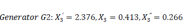
Table 1: Generator parameters

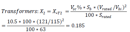
Table 2: Transformer parameters
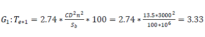
Transmission line parameters: Voltage = 110KV,
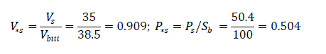
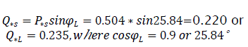
Cosφ = 0.90, System voltage Vs = 35KV, line length = 50km,
Short circuit line length (from source) = 15km,
System power = 50.4 MW, Short circuit switch off time tsw = 0.15 sec., re-closure time tr = 0.1 sec.
(1) To find static stability of the power system.
(2) To calculate dynamic stability of power system.
(3) To find the influence of auto re-closure on dynamic stability of transmission lines.
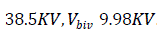
There are four sub-divisions of voltage level as can be seen from Fig.1.0. The calculation is done in per unit value taking the base values as Sb = 100 MVA and Vb = VbII = 115 KV. The base values of the remaining sections are: 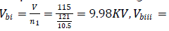
Similarly, 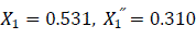
Similarly, 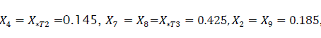 Fig. 2.0.
Line Parameters  where per unit reactance of aluminium conductor is 0.4 ohm/km [1].
Short circuit inductances X1k=(35/50)*0.151=0.1057; X2k=(15/50)*0.151=0.0453, where 50km = total line length and 15km=short circuit line length.
Similarly, 
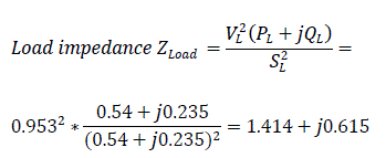
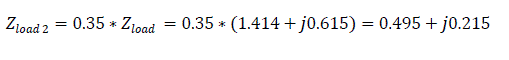
Load power is 54MW =(0.54+j0.235)
The next step is to simplify Fig. 2.0.
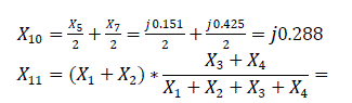

Figure 1: Circuit diagram of transmission lines

Figure 2: Impedance diagram of the transmission lines shown in figure 1

Figure 3: Simplified impedance diagram
The total voltage at the system bus bar is 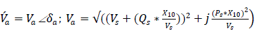

Voltage at the load bus bar
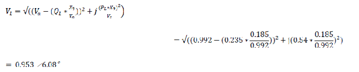
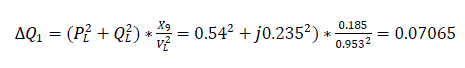
Loss of reactive power in the inductances of X9 and X10
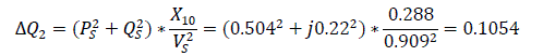
Over all power available in the system
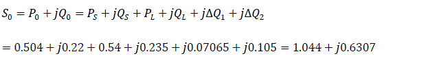
The power generated by the turbine is P0=1.044
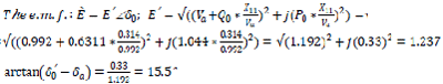
The angle between emf E' and system voltage 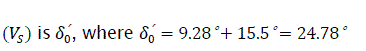
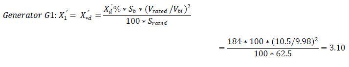
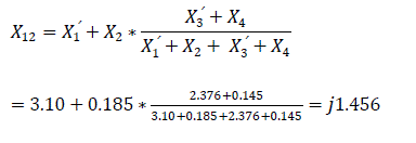
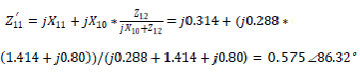
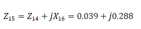
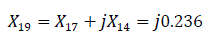
The synchronous emf Eq ∠ δ'0 will be defined. For this purpose, the schematic impedance diagram of Fig. 2.0 will be adjusted by replacing the transient reactance X'd of the generator with the synchronous reactance Xd value. Therefore Fig. 3.0 will express X12 as:
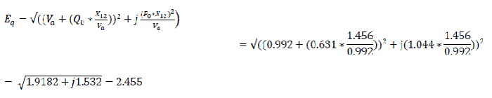
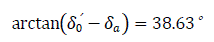
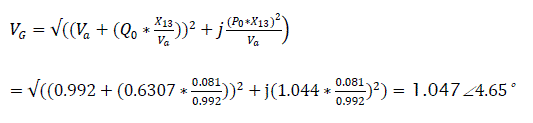
The angle between emf Eq and system voltage Vs is δ'1=38.63°+9.28°=47.91° Voltage VG on the busbar of the equivalent diagram of generator excluding the generator resistance is represented by Fig. 2.0.

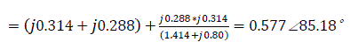
a) Without auto regulation of excitation system the self inductance Z'11 will be:
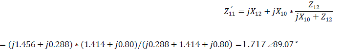
The corresponding self impedance angle 
Self admittance of the circuit 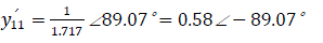
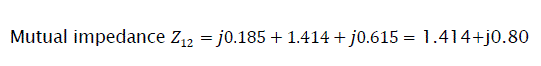
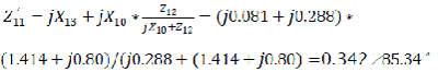
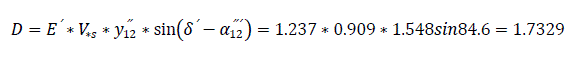
Mutual impedance of the current
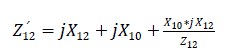
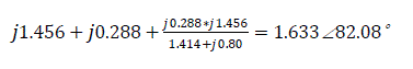
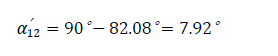
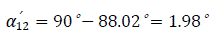
The corresponding mutual admittance angle
Mutual admittance 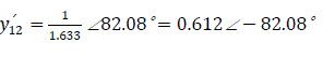
b) With the presence of semi-automatic excitation regulator, the impedance becomes:
The corresponding angle 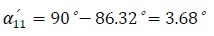
Self admittance 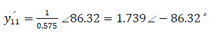
Mutual impedance 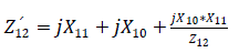

c) With the presence of automatic excitation regulator:
The corresponding self impedance angle 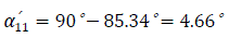
Self admittance of the circuit 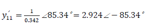
Mutual impedance 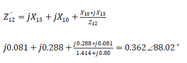
Mutual admittance 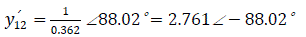
In determining the shunt resistance created by one phase short circuit to ground, the diagram of Fig. 4.0 will be applied for reverse and zero sequences.

Figure 4: System reverse sequence impedance diagram
For reverse sequence, load resistance is taken as 0.35Zload [2], therefore:
Rearranging the diagram of Fig. 4.0, it becomes:
Impedance transformation of figures 5 and 6
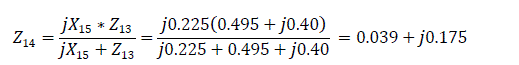
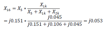
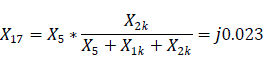
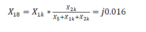

Figure 5: Δ/Y impedance conversion

Figure 6: Resultant impedance from Figure 5
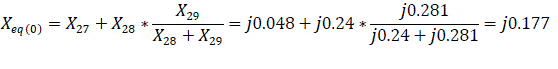
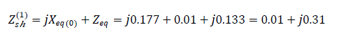
The equivalent impedance of the reverse sequence relative to the short circuit is Zeq.
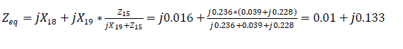

Figure 7: Zero sequence impedance diagram
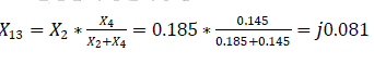
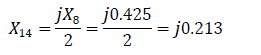
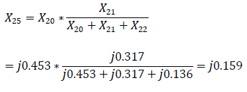
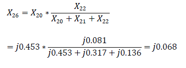
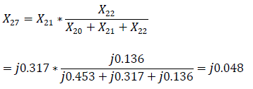
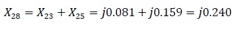
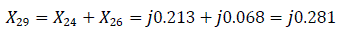
For transmission lines, zero sequence reactance is defined as X0 = 3X1 [3]. Similarly, X20=3X5; X21=3X1k; X22=3X2k; X23=X2*X4/(X2+X4) = 0.0185*0.145/(0.0185+0.145) = j0.081
X24 = jX7/2 = j0.425/2 = j0.213 (Fig. 7.0).

Figure 8: Conversion of Δ/Y impedance diagram
The equivalent reactance of the zero sequence relative to the point of short circuit K(1) is defined as:
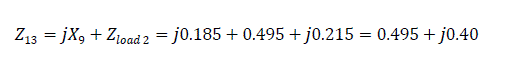
The impedance of the power line at the point of short circuit is:
Abnormal regime
Calculation of system reactance for single line-to-ground short circuit at15km distance from source.
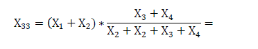
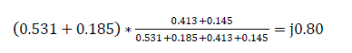
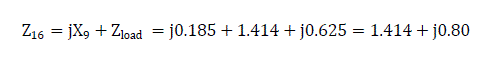

Figure 9: Abnormal regime impedance diagram
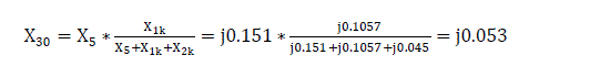
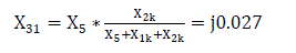
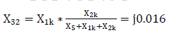
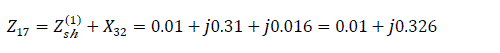
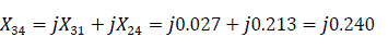

Figure 10: Equivalent generator circuit
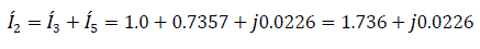
Current quantity and its flow during abnormal regime Fig. 10
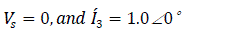


Input emf 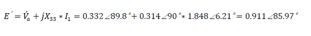
Self impedance: 
Self admittance angle: 
Self admittance 
Mutual admittance 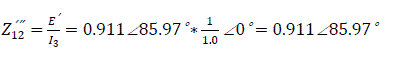
Mutual impedance angle: 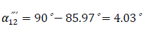
Mutual admittance: 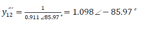
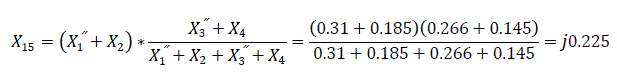
Self and mutual reactance after accidental regime
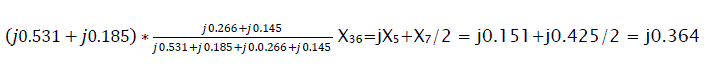
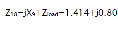

Figure 11a: Reactances after accidental regime

Figure 11b: Equivalent diagram after accidental regime
Self impedance: 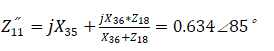
Self admittance angle: 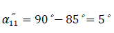
Self admittance: 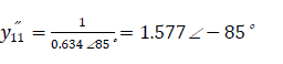
Mutual impedance: 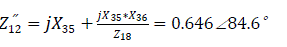
Self admittance angle: 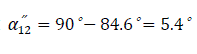
Self admittance: 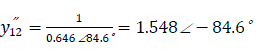
(a) Without automatic excitation regulator on generator

(b) With semi-automatic excitation regulator

(c) With automatic excitation regulator

6. Calculation of power characteristics at different regimes:
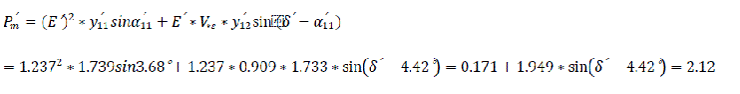
1) Maximum power at normal regime
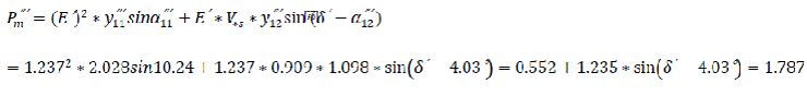
2) Maximum power at faulty regime
3) Maximum power after fault clearance
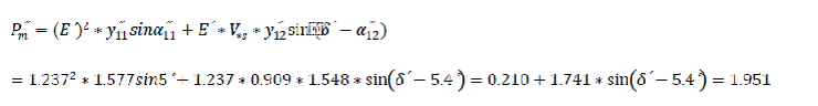
Taking values of δ′ from 0° to 180°, the values of Pm′ ,Pm″′,and Pm″ will be calculated as shown in Table 3.

Table 3: Values of 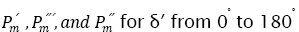
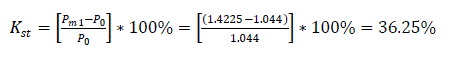
Static stability at normal regime without auto-regulation of excitation
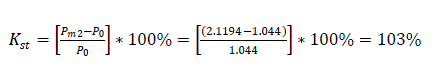
Static stability at normal regime with semi-automatic regulation of excitation
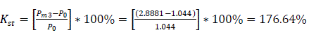
Static stability at normal regime with automatic regulation of excitation
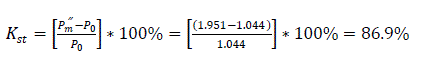
Static stability regime after fault clearance
For three phase short circuit Pm″′=0 4 . The limit of switch off angle δlim of the short circuit is defined thus:
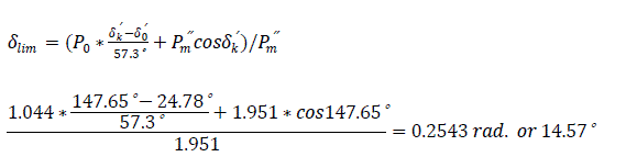
where 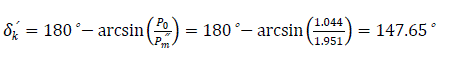
The coefficient 57.3° converts degrees to radians.
Determination of switch off angle as a function of switch off time δ′=f(t) can be drawn by taking intervals of t=0.15 at Δt=0.05 second.
First interval Δt=0 to 0.05 second
Electrical power given out at the first moment after the short circuit is Pm″′=0, this is because there will be no system voltage Vs during three phase short circuit. Power at the initial interval is P0 =1.044. Increase in angle for this interval is:
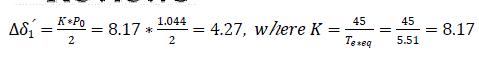
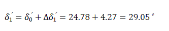
Second interval Δt=0.05 to 0.1 second, ΔP1 =P0 =1.044
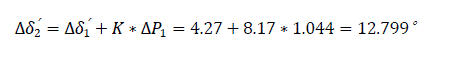
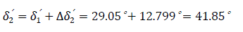
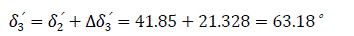
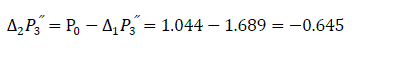
Third interval Δt=0.1 to 0.15 second, ΔP2 =1.044 (switch off time)

Forth interval Δt=0.15 to 0.20 second, ΔP3 =1.044 (first power imbalance)
For this interval, the switch off of the short circuit begins. The electrical power given out after the accident in the beginning of the forth interval will be:
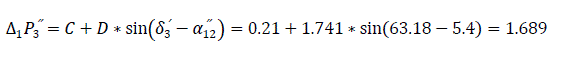
Where 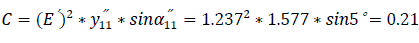
Second power imbalance at the beginning of the forth interval
Increase in angle for this interval:
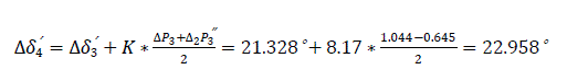
Angle at the end of the forth interval
Fifth interval at Δt = 0.2 to 0.25 second
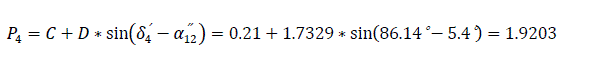
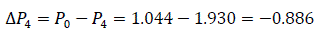
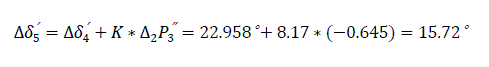
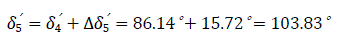

Table 4: Results of δ′ = f(t)
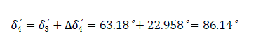
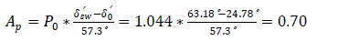
Table 4.0 is illustrated in Fig. 12.0, showing (δ0′=24.78°) angle between the emf and the system voltage. δsw′= δ3′=63.18° - the switch off angle at t=0.15 second. δr′=δ5′= 103.83° – retardation angle at the elapsed time (re-closure angle).

Figure 12: Generator swing curve
Speed up area Ap and possible retardation area Ar are defined in Fig. 13.0

Reserved coefficient of dynamic stability of the power system (Kr) is defined as 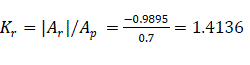

Figure 13: Dynamic stability curve
The influence of a successful auto-reclosure on the dynamic stability of the system has been presented. From table 4, it is seen that reclosure angle δr′ is equal to 103.83° and reclosure time is 0.1second. Therefore, the retardation areas before Ar1 and Ar2 can be defined as stated below. These parameters can be used to define the coefficient of dynamic stability of the system through the influence of auto-reclosure equipment installed on the power system.


Finally, the coefficient of dynamic stability of the system 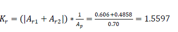
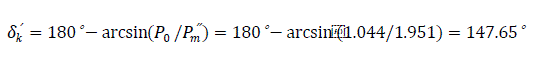
As a result of the presence of automatic re-closure system on the power line, the re-closure angle was improved to 147.65°. Consequently, the coefficient of dynamic stability was raised to 1.5597 as compared with the 1.4136 earlier obtained after fault clearance. This result proves that the reserve of dynamic stability with auto re-closure in the system is more than when there is no auto re-closure system on the transmission line. Therefore, a successful automatic re-closure of transmission lines positively influences the dynamic stability of power systems.