Research & Reviews: Journal of Pure and Applied Physics
ISSN: 2320-2459
ISSN: 2320-2459
1Czech Technical University, Czech Republic
2Open University of Cyprus, Cyprus
Received Date: 18/05/2017; Accepted Date: 16/06/2017; Published Date: 26/06/2017
Visit for more related articles at Research & Reviews: Journal of Pure and Applied Physics
We consider quantum systems in d dimensional Hilbert space using a computational approach. We focus on a specific analytic representation in a cell S which describes the finite quantum system. The time evolution of the system produces d paths of zeros. The central notion is to restrict our attention to matrices such as: Vandermonde and Banded instead of any periodic Hamiltonian matrix. In particular we provide numerical examples of interesting closed paths of the zeros. In this paper we use an efficient numerical approach to generate the paths of zeros based on specific categories of matrices
Harmonic oscillator, Quantum system, Logarithmic functions
An analytic representation in finite quantum systems [1-7] which is represents a state in d-dimensional Hilbert space. Various analytic representations [8-11] have been studied in quantum mechanics. The most popular analytic representation is the Bargmann representation in the complex plane for the harmonic oscillator [12-14], One of the most important aspect in the theory of analytic functions [15-18] are zeros and the paths of the zeros [19-21]. In d-dimensional Hilbert space, the zeros define the state uniquely. The zeros of analytic functions in a square cell S is equal to d and the zeros obey a constraint [22-24].
So far periodic Hamiltonian matrices were used to study the quantum system. In this paper we study the paths of the zeros using some important types of matrices as: Vandermonde and Banded. This matrix belongs to a more restricted category of the matrices that can be used to understand the behavior of the d paths of the zeros of the finite quantum system. Vandermonde matrices exist only when d=3. When d>3 Vandermonde matrices are not periodic, unless the identity matrix, and therefore cannot be used for our situation. Needless to say that the evaluation of such inverse matrices is a key point to study for our quantum system. For example to find functions of a matrix, such as exponential functions (evolution operators) and logarithmic functions (entropies) is important for the study of quantum mechanical topics. This result can be used to improve the problem of the behavior of paths of the zeros which have properties uniquely determined by Banded and Vandermonde matrices. We prove numerically that the paths of the zeros under this quantum system produces graph which enable us to determine the acceleration and velocity of the system.
The following question is examined: Is it possible to understand the paths of the zeros using these types of matrices (Vandermonde and Banded)? We will show numerically that there exist cases where the paths of the zeros of one Vandemorde matrix and one Banded matrix have the same multiplicity.
In section II, we give a brief introduction in finite quantum systems. We introduce an analytic function for these systems.
In section III we study the zeros of the analytic representation. The paths of the zeros during time evolution are considered. In the case of matrices with rational ratio of the eigenvalues (so that there exists t with exp (itM)=1) the system is periodic and the paths of the zeros follow a closed curve. Our new results are summarized in this section where we plot the paths of the zeros using Vandemorde and Banded matrices and explaining their importance.
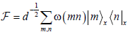
We consider a finite quantum system with variables in Z(d) (where d is an odd integer). It is described with the d-dimensional Hilbert space H(d). Suppose |m)x be the position and |m)p be the momentum bases (where m ∈ Z(d)). We define the Finite Fourier transform as follows:
 (1)
(1)
Where 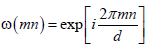 . The position and momentum states are related through a Fourier transform, as follows:
 (2)
(2)
We assume that  is an arbitrary normalized state.
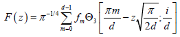
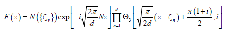
We define the analytic represesantion of the state , [22, 23]
 (4)
(4)
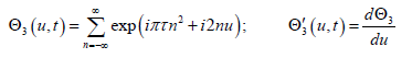
where Θ3 is the Theta function,
 (5)
(5)
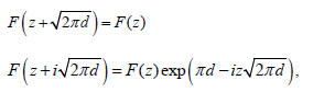
The quasiperiodicity relations for the analytic function F (z) are:
 (6)
(6)
and therefore this function is defined in a cell.
 (7)
(7)
Where M and N are integers that defined the cell S. The analytic formalism of eqn. (4), can be used in order to study the completeness of finite sets of coherent states in the cell S.
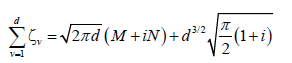
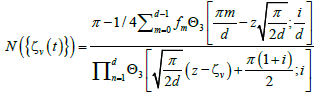
In finite Hilbert space, the analytic function F (z) has exactly d zeros ζv in each cell S, and the following constraint.
 (8)
(8)
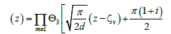
in finite systems the d − 1 zeros define uniquely the state (the last zero is determined from eqn. (8)). In infinite systems the zeros do not define uniquely the state. The function F (z) is also given by:
 (9)
(9)
Here N is the integer that labels the cell (as in eqn. (8)), and  is a normalization condition. Below we choose the cell with N=0. The proof of eqns. (8) and (9) is given in refs. [22-24].
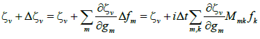
Let M be a matrix of the system (a d × d Hermitian matrix Mmn). As the system evolves in time t, each zero ζv follows a path  .
.
We want study the actual path using matrices with various properties and we compute the analytical expressions for the derivatives of the functions ζv (f0,..., fd−1) in matlab. Therefore, we plot the graphs using the following equation:
 (10)
(10)
Where,
 (11)
(11)
And,
 (12)
(12)
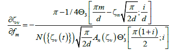
In each step of the iteration process,  is calculated as:
 (13)
(13)
The proof of eqns. (10)-(13) is given in ref. [19].
We consider periodic systems such that  for some T. This is a periodic system iff the ratios of the eigenvalues of
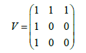
  are rational numbers. We say the path of the zeros have K multiplicity when a number K of the zeros follow the same path. An example is the following Vandemonde matrix:
 (14)
(14)
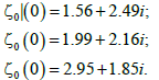
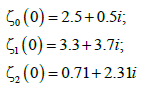
The period of Vandermonde matrix is T=2π. At t=0 the zeros are the following:
 (15)
(15)
Based on general eqn. (10) we generate the paths of the zeros.
The paths of zeros which are satisfied by eqn. (15), are shown in Figure 1. In Figure 1 using the zeros of eqn. (15) with the Vandemorde matrix eqn. (14), it can be observed that the zeros follow a closed path, resulting to  . As a result, the multiplicity of the path of the zeros equals to 3, (M=3). In the graph it can be seen that the ζ0 (t) after a period of t=2π occupies the position of the ζ0 (t). For the ζ1 (t) after a period of t=2π occupies the position of the ζ2 (0) and finally for the ζ2 (t) after a period of t=2π occupies the position of the ζ0 (0). The ZR values (real the values of the zeros) are represented in the horintal axes. The ZI values (imaginary the values of the zeros) are represented in the vertical axes.

Figure 1: Paths of the zeros using the matrix of eqn. (14). At t=0 the zeros are given in eqn. (15).
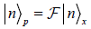
We also consider another Vandermonde matrix:
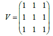 (16)
(16)
In this case the period is T=π. We consider the following set of zeros:
 (17)
(17)
In a period of 2π, using the zeros of eqn. (17) and Vandemorde matrix of eqn. (16), the zeros follow their own path with a multiplicity equal to 1, (M=1). In Figure 2 the paths of these zeros are demonstrated.

Figure 2: Paths of the zeros using the matrix of eqn. (16). The zeros at t=0 are given in eqn. (17).
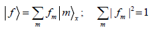
We consider the following banded matrix:
 (18)
(18)
In this case the period is T=2π. We consider the following set of the following zeros:
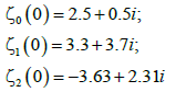 (19)
(19)
The paths of zeros using the zeros in eqn. (19) and the matrix of eqn. (18), are shown in Figure 3. It can be concluded that the zeros follow a closed path, resulting to  . Therefore, the multiplicity of the path of the zeros equals to 3, (M=3). Using the zeros of eqn. (15) and the Banded matrix of eqn. (18), the paths of the zeros are shown in Figure 3.

Figure 3: Paths of the zeros using the matrix of eqn. (18). The zeros at t=0 are given in eqn. (19).
We have studied quantum systems in d - dimensional Hilbert space with phase space Z(d) × Z(d). In eqn. (4) an analytic representation of these systems in terms of Theta function is defined. In finite quantum systems the d zeros defines the quantum state uniquely.
The d paths of the zeros are used to describe the time evolution of the system. Using eqn. (10) we produce the paths of the zeros. The motion of the d paths of the zeros using special case of matrices is studied. Some examples of the paths of the zeros using Vandemorde and Banded matrices are given.
There is a connection between the zeros of analytic functions and the quantum systems. In finite quantum systems the zeros define the state of the system and the paths of the zeros are in d paths on a torus. The Hamiltonians that we are using are periodic so the zeros follow closed paths. Our goal was to find specific cases of matrices that we can explain in more detail the behaviour of the paths of the zeros. We have assumed that there exist specific cases of periodic Hamiltonians which give as better understanding of the behaviour of the paths of d zeros (Appendix).
In conclusion we have study the quantum systems by looking at the behaviour of the paths of the zeros. This is important because if we know the behaviour of the paths of the zeros we will be able to find the acceleration and the velocity of the paths of the zeros. That means we can understand the quantum system completely when the time evolves. We have produce results using Vandemonde and Banded matrices for first time. The contribution of this work since these matrices produces new type of solutions which can have physical meaning.