On New Generalized Logistic Distributions and Applications Barreto FHS, Mota JMA and Rathie PN*

Abstract

In 2006, Rathie and Swamee had proposed a generalization of the logistic distribution which is more flexible and multimodal. This work presents an addition of a new parameter to increase the flexibilization of the distribution as well as an asymmetric distribution using the Azzalini method, adding another parameter of asymmetry. Five data sets (Human Body Fat Index, HIV, Precipitation, pH Concentration, Relative Humidity) are analysed by applying the new distributions. The estimation of the parameters of the new distributions and mixture of the normals was accomplished by the automaximum likelihood method. Due to complex mathematical resources required to calculate the estimates of the new distributions, we use interactive numerical methods such as L-BFGS-B, BFGS, SANN etc. using an adaptive barrier algorithm added to enforce the constraint and an adapted function that searches for global maximum of a very complex non-linear objective function to initial values of the algorithm of estimation. All computational work was implemented in software R. In most cases, we use the Hartigan’s test to reject unimodality. Using the KolmogorovSmirnov test at significance level of 5% and applying various criteria, such as Mean Square Error, Mean Absolute Deviation and Maximum Deviation, to indicate the best fit. The classical and general method for multimodal adjustment is a mixture of distributions, in particular, the mixture of the normal distributions because the normal distribution presents good mathematical properties. In the case of mixture of the normals, we use EM algorithm to calculate the estimates. We also use Akaike Information Criterion and Bayesian Information Criterion as selection criteria to highlight the best distribution, in both cases, comparing them with the mixture of normal distributions to illustrate the applicability of the results derived in this paper.

Keywords

Rathie-Swamee distribution, Azzalini method, multimodal data set analysis, Akaike criterion information, Bayesian criterion information, maximum likelihood method, Kolmogorov-Smirnov test

Introduction

There are several classical models, such as normal, exponential, binomial, Poisson, logistic etc. to analyze different data sets. As there is not a single unified model, we have to construct new models suitable for the data sets under consideration. The logistic model is very useful in many areas in statistics and physics. This article is divided as follows: Section 2 deals with symmetric generalized logistic distribution whereas in Section 3 the skew form is studied. Section 4 presents applications to analyze five real data sets using the results of earlier sections and comparing them with the mixture of two normal distributions where possible. The article ends with a short conclusion and a list of references. Rathie et al.[1] defined a multimodal symmetric distribution function G(x) for a random variable X∼RS (a, b, p) as

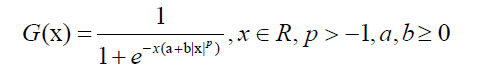1

With a and b not zeros simultaneously. For b=0 or when p=0, (1) is written as a logistic distribution

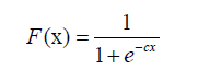2

Where c=a or c=a + b. The density function corresponding to (1) is

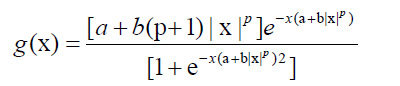3

Generalized Symmetric Logistic Distribution

A symmetric distribution can be generated by using the method proposed by Jones in 2004 [2]. Let U ~Beta (α,α), and X=G- ¹(U), where G(x) is a distribution function of g(x). Then, the distribution function H(x) of X is given as

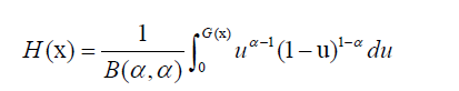4

Differentiating H(x) yields the corresponding density function as

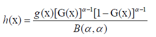5

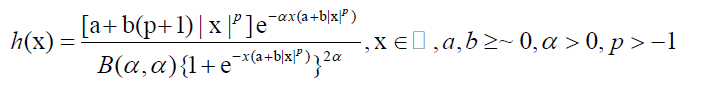
Using (1) and (3) in (5), the generalized symmetric logistic density function for X ~ RSG (a, b, p, α) is given by

6

Where both a and b not zeros simultaneously and B (., .) is the beta function. For α=1, reduce to (3). We may introduce the location parameter μ in the model (6). There is no need to introduce the scale parameter, otherwise the density function will become non-identifiable. The density function (6) takes the following form on introducing the location parameter μ є R:

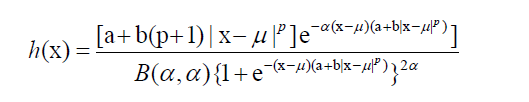7

The Figures 1 to 4 show graphs for (6) and (7) respectively for various values of the parameters μ, a, b, p and α.

Figure 1: Graphs of (6) and (7) for Fixed a.

Figure 2: Graphs of (6) and (7) for fixed b.

Figure 3: Graphs to (6) and (7) for fixed p.

Figure 4: Graphs of (6) and (7) for fixed α.

Distribution function

In this subsection, we prove that the distribution function corresponding to (6) is given by

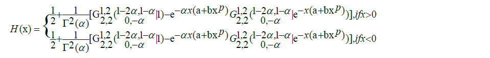8

Proof. For x > 0, we have

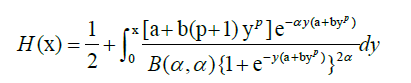9

Substuting 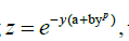we get

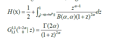
we have

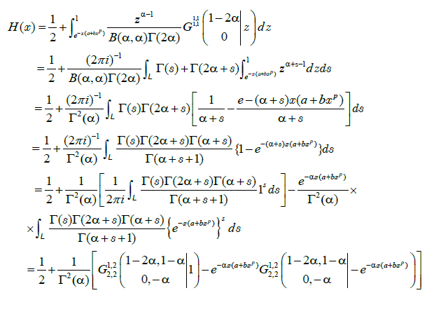10

By symmetry, we easily write the result for x < 0.

Moments

In this subsection, we obtain the n-th moments about the origin. By definition,

when n is an even integer

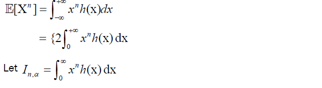11

Then, by expanding the denominator by binomial theorem, we have

12

when n is an even integer.

The variance of X ~ RSG (a, b, p, α) is given by

13

Generalized Skew Logistic Distribution

In Azzalini density [3]

s(x) = 2 v(x)V[w(x)], x∈R 14

With w(x)=kx; k 2 R, take v(x) as the density function of X ~ RSG(a; b; p; ) and V (x) as the distribution function of X ~ RS(a; b; p). Then, the density function of generalized skew logistic model X ~ RSGA (a; b; p;α; k) is given by

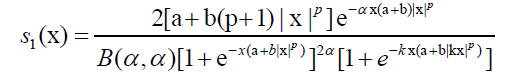15

Introducing the location parameter μ∈^R, the density function of X ∼ RSGA (a, b, p, α, k) is given by

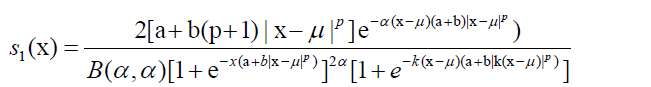16

For certain values of the parameters, s(x) and s1(x) are plotted in Figure 5 for k =±0.7 and in Figures 6 and 7 for a=0 and b=0 respectively.

Figure 5: Graphs of (15) and (16) for certain values of the parameters.

Figure 6: Graphs of (15) and (16) for certain values of the parameters with a=0.

Figure 7: Graphs of (15) and (16) for certain values of the parameters with b=0.

Applications Involving Real Data

In the present section, five data sets are analyzed by using the distributions defined in earlier sections as well as the mixture of two normals for bimodal data. The estimation of parameters is done by utilizing the method of maximum likelihood estimation. Akaike Cri- terion Information [4], Bayesian Information Criterion, Mean Square Error, Absolute Mean Deviation and Maximum Absolute Deviation are calculated to judge the fit of RSG, RSGA and mixture of two normals. The goodness of fit test of Kolmogorov-Smirnov is used with significance level of 5%. Some packages of sotfware R are used. The GenSA package [5] is used to obtain initial values to interactive algorithm. For interactive algorithm, we use the bbmle::mle2 package [6], in most cases, using BFGS method and optimizer constrOptim to guarantee that the estimated parameters are consistent within their respective parametric space. For more details to adaptive barrier algorithm, see stats::constrOptim into soft- ware R. We obtain the estimates of the parameters, approximate the standard errors of the estimates based on quadratic approximation to the curvature at the maximum likelihood estimate, and a test (z test) of the parameter difference from zero based on this standard error and on an assumption that the sampling distribution of the estimated parameters is normal.

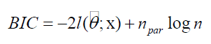
The AIC and BIC for the classification of the model-fit on data sets in various applications will be used. These are defined below

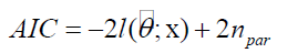17

where ņ_par is the number of parameters to be estimated and l(.;.) is the logarithm of the estimated likelihood function.

18

where η is the number of observations. Mean Square Error (MSE), Mean Absolute Deviation (MAD) and Maximum Absolute Deviation (MD) are defined below:

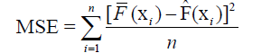
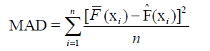
where is the empirical cumulative distribution and is the fitted cumulative distribution of the data. Of course, the smallest value obtained will indicate that there is a good fit.

Human body fat index

The data consist of 252 observations on 17 variables about human body fat. For details, see Jonhson [7], Penrose et al. [8], and Ambler et al. [9]. Figure 8 demonstrates that the data is unimodal which is also confirmed by test [10,11] with statistics D=0.014114 and p-value near 1. The estimates of the parameters using RSG and RSGA models are given in Table 1.

Table 1: Estimates associated with RSG and RSGA models.

Figure 8: Adjustments of two new distributions to Body Fat Index.

Table 2 shows the comparison of the models used. Figure 8 presents the histogram with adjusted models. The empirical and theoretical distributions are shows in Figure 9.

Table 2: The comparison of adjusted models used.

Figure 9: Graphs of empirical and theoretical distributions..

For AIC, it may be observed that the RSGA fit is better than RSG fit for this data set. The Bayesian criterion indicates a better fit for RSG distribution.

Precipitation

The data consist of 121 observations about annual precipitation (rain) between 1978 and 1998 at the center of the city of Los Angeles. These data were obtained from the site [12]. Figure 10 demonstrates that the data is unimodal which is also confirmed by Hartigan’s test with statistics D=0.027273 and p-value equal to 0.7971. The estimates of the parameters, using RSGA distribution, are given in Table 3.

Table 3: Estimates associated with RSGA model.

Figure 10: Graphs of empirical and theoretical distributions.

Applying the non-parametric Kolmogorov-Smirnov test, the K-S value obtained is 0.07438 with p-value 0.8914, thus not reject the hypothesis that the data satisfies RSGA distribu- tion. In 2014, Eirado et al. [13] proposed an asymmetric model and applied to this data set. The MSE obtained is equal to 0.001058396, the mean absolute deviation (MAD) is 0.02785116 and the maximum absolute deviation (MD) is 0.06496284. Also, we obtained MSE equal to 0.0002414233, MAD equal to 0.01185483 and MD equal to 0.04669135.

AIC and BIC of the fits of the two models are given in Table 3,4. The empirical and theoretical distributions are shows in Figure 11. Clearly, the RSGA distribution gave better fit to the precipitation data.

Table 4: The comparison of the models.

Figure 11: Empirical and theoretical distributions of precipitation.

HIV Data

The HIV data with 2843 observations is available in fitdistrplus: Aids2 package of software R, giving the age when a patient is diagnosed with AIDS in Australia in 1991. Table 5 presents the estimates of the parameters of RSG and RSGA models.

Table 5: Estimates associated with RSGA and RSG models.

Table 6: Estimates associated with asymmetric normal and normal distributions.

Histogram and RSGA distributions to HIV data are shown in Figure 12 while Empirical and RSGA distributions in Figure 13. In Table 7, the Kolmogorov-Smirnov test rejects almost all adjusted distributions except RSGA distribution.

Figure 12: Adjustments of RSGA distribution to HIV data.

Table 7: Comparison of the models used. Comparison of the models used.

Figure 13: Empirical and theoretical distributions to HIV data.

pH Concentration data

The pH concentration data [14] with 252 observations show bimodality which is also demonstrated by Hartigan’s test with statistics of the test equal to 0.046498 and p-value of 0.00045. The estimates of the parameters are given in Table 8.

Table 8: Estimates associated with RSGA and RSG models.

Silva et al. [15] proposed two new asymmetric models by Azzalini’s method h1(x) and h2(x) where the pH concentration data was fitted by these two models. Table 10 shows the performance of the fitted distributions.

Using package of Benaglia et al. [16], the estimates of mixture of normals are given in Table 9 with parametric bootstrap performed for standard error approximation.

Table 9: Estimates of mixture of two normal.

Histogram of pH values along with the distributions adjusted are shown in Figures 14 and 15

Figure 14: pH histogram and the fitted models.

Figure 15: Graphs of empirical and theoretical distributions.

Table 10 gives the accuracy values of AIC, BIC, MSE etc, for various models. The RSG model adjusted well the bimodal data.

Table 10: Comparison of the models used.

Relative Humidity (RH)

The RH observations data are taken from Nychka et al. [17]. The estimates of the parameters for RH data using the RSGA model are given in Table 11.

Table 11: Estimation of the parameters of the RSGA model.

The estimation for a mixture of two normal s are given in Table 12. The values of AIC, BIC etc. measuring the quality of fit are given in Table 13.

Table 12: Estimation of the parameters of the mixture of two normal.

Table 13: Comparison of the models used,

In Figure 16, the histogram and the fit using Empirical, RSGA and the mixture of two normals distributions are shown. In Figure 17, the empirical and theoretical distributions are shown.

Figure 16: Relative Humidity and adjusted model.

Figure 17: The empirical and theoretical distributions.

Conclusion

The Rathie-Swamee generalized distribution (RSG) and its skew form (RSGA) proved useful to five data sets analyzed, thus demonstrating their applicabilities over the mixture of two normals, in case of bimodal sets (pH concentration and relative humidity).

Acknowledgement

P. N. Rathie thanks the Coordination for the Improvement of Higher Level Personnel (CAPES) for supporting his Senior National Visiting Professorship.

References

1. Rathie PN, et al. On a new invertible generalized logistic distribution approximation to normal distribution, technical research report in statistics. Applisciephy. 2006;1:120-125.
2. Jones M, et al. Families of distributions arising from distributions of order statistics. Test.2004;13:1-43.
3. Azzalini A. A class of distributions which includes the normal ones. Scand J Stat Theory. 1985;12:171-178.
4. Akaike RW.A new look at the statistical model identication. IEEE Trans Automat Contr. 1974;19:716-723.
5. Xiang Y, et al.Generalized simulated annealing for ecient global optimization: the GenSA package. R J. 2013;5:13-28.
6. https://rdrr.io/cran/bbmle/
7. Johnson RW and Carleton C. Fitting percentage of body fat to simple body measurements. J Stat Educ. 1996;4:265-266.
8. Penrose KW, et al. Generalized body composition prediction equation for men using simple measurement techniques, Med ScieSpo Exe. 1985;17:1-8.
9. https://cran.r-project.org/web/packages/mfp/index.html
10. Hartigan JA and Hartigan PM. The dip test of unimodality. Ann Stat.1985;13:70-84.
11. https://cran.r-project.org/web/packages/diptest/index.html
12. http://www.noaa.gov/
13. Eirado CRDR and Rathie PN. On new invertible skew and symmetric distributions. StatRese Lett.2014;3:17-22.
14. Growitz DJ, et al. Reconnaissance of mine drainage in the coal elds of eastern Pennsylvania. TechRep US Geological Survey. 1985.
15. Silva RO, et al. On the new skew distributions using azzalinis formula. MathematicaAeterna. 2016;6:649-673.
16. Benaglia T, et al. Mixtools: An R package for analyzing nite mixture models. J Stat Softw.2009;32:1-29.
17. Nychka D, et al. Tools for plotting skew-T diagrams and wind profiles, R package version. 2014;1.4.