Research & Reviews: Journal of Pure and Applied Physics
ISSN: 2320-2459
ISSN: 2320-2459
Paul Bracken*
Department of Mathematics, University of Texas, Texas, USA
Received: 08-Jan-2024, Manuscript No. JPAP-24- 124668; Editor assigned: 11- Jan-2024, Pre QC No. JPAP- 24-124668 (PQ); Reviewed: 25-Jan-2024, QC No. JPAP-24- 124668; Revised: 01-Feb- 2024, Manuscript No. JPAP- 24-124668 (R) Published: 08- Feb-2024, DOI:10.4172/2320- 2459.12.1.002.
Citation: Bracken P, Decoherence in Atom-Field Interactions and Quantum Entropy. Res Rev J Pure Appl Phys. 2024;12:002.
Copyright: © 2024 Bracken P. This is an open-access article distributed under the terms of the Creative Commons Attribution License, which permits unrestricted use, distribution, and reproduction in any medium, provided the original author and source are credited.
Visit for more related articles at Research & Reviews: Journal of Pure and Applied Physics
The concept of decoherence is introduced and studied in some situations in which there is an atom-field interaction. This type of physical model can be applied to the areas of quantum optics, information processing and computing. It offers the opportunity to observe how unitarity is affected by decoherence. A master equation is solved for the density matrix in a rigorous manner which can be used to calculate system entropy. Pure states and mixtures can also be discussed based on this.
Quantum; Algebra; Eigenvalue; Matrix
The relationship between the macroscopic and microscopic is an area of great interest in quantum mechanics. A conflict seems to exist between these two length scales. One approach put forward by Caldeira and Legget is based on the observation that all quantum mechanical systems are part of or embedded inside a much larger system with many degrees of freedom, which is usually called a reservoir. The interaction of a quantum system with a reservoir or bath means that quantum coherence can decay. An embedded quantum system is referred to as an open system [1-9].
The interaction of a quantum system with a much larger reservoir has the consequence that quantum coherence in the quantum system decay away.
This process is called decoherence and occurs as an intrinsic, important part of quantum mechanics. It comes up, for example, in quantum optics. As a short introduction to decoherence and de-phasing, suppose a two-level quantum system S is described by,
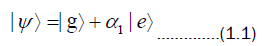
The states  represent an arbitrary basis called ground and excited, respectively. A two level atom will be
introduced shortly. Suppose S interacts with a large reservoir R whose state can be expanded with respect to an
orthonormal basis called
represent an arbitrary basis called ground and excited, respectively. A two level atom will be
introduced shortly. Suppose S interacts with a large reservoir R whose state can be expanded with respect to an
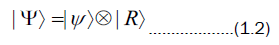
orthonormal basis called  Initially, the state of the combined system S+R is described by a separable state
which can be factored,
Initially, the state of the combined system S+R is described by a separable state
which can be factored,
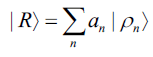
such that an initial state for the reservoir is,
However, due to some interaction, the state of the combined system no longer stays factorized as indicated in (1.2), in fact,
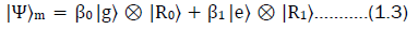
In (1.3)  are other normalized states of the reservoir such that
  The reduced density matrix
 corresponding to (1.3) takes the form

To determine a density matrix that only pertains to S, the terms relevant to the reservoir in (1.4) must be traced out. Using the orthonormal basis for R we can expand
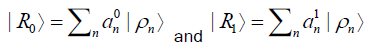 the trace is found to be
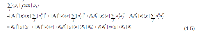
The fact that 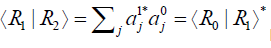 In matrix form this reduced density matrix is given by
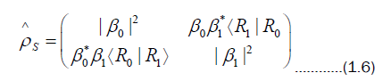
It is apparent that the diagonal elements have not been altered by this procedure, whereas the off-diagonal elements are now multiplied by a number such that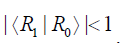 The diagonal elements of the reduced density matrix remain invariant only because the energy dissipation takes place over a longer time scale than decoherence.
An atom field interaction serves as a model for this idea and leads to a realization of quantized field measurements. The measurement of the ground and excited states will provide information about the field state. The field can also be regarded as a type of both. Atoms passing through the cavity acquire knowledge of the field by means of its entanglement with it and as they depart the cavity, it is possible this information may be retrieved.
Decoherence and the entropy increase are linked. As with von Neumann’s projection, the decoherence mechanism serves to eliminate the cross terms. Decoherence could provide a physical mechanism to realize the projection. Decoherence is the loss of coherence between the component of a superposition in terms of the action of an external environment on the coupling between system and apparatus [10-13].
The main objective here is to investigate some aspects of decoherence as introduced here in atom-field interactions and its relationship with entropy and other things of physical interest. It is intended the systems studied here and the work done with them will yield more insight into the relationship between quantum and classical integrability. The properties of open systems also come up. Although the systems which are considered may be quite different, the plan is to study each of them by means of similar, related methods [14-17].
Quasi-classical interactions
Atoms provide a means of obtaining information about quantum properties of the electromagnetic field, and atom
field interaction can be studied by means of a number of different approaches. It is worth starting with a quasiclassical
model to provide a contrast to the fully quantum cases to be studied next. With respect to the discrete
spectrum of an atom, two of the energy levels may be connected by a near resonant transition initiated by a
monochromatic electromagnetic field. The two levels of the atom are  excited as above. Let us
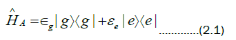
associate energies ε g and εe with the ground and excited state of a two level atom. The atomic part of the
unperturbed Hamiltonian can be written as
excited as above. Let us
associate energies ε g and εe with the ground and excited state of a two level atom. The atomic part of the
unperturbed Hamiltonian can be written as
To place the origin between the two levels we can add the term  and subtract
 to both sides of (2.1) so we can use
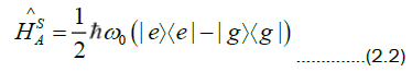
where 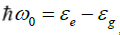 and an overall constant has been dropped.
The interaction Hamiltonian between the atom and field is assumed to be dipole and the electromagnetic field is not quantized.The interaction is 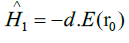 where d is the atomic dipole moment and E(r0) the electromagnetic electric field evaluated at r0, the position of the dipole. Assuming the states
  have definite parity, the matrix elements of the dipole operator have to be off-diagonal, that is,

A Hamiltonian for the atom-field interaction is modelled by
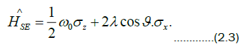
In (2.3),  , where ω is the field frequency and
  are Pauli matrices. Explicit time dependence has
been given to the harmonic term and λ =|G|E0/2 is a real interaction constant, E0 the field amplitude. The Pauli
matrices and basis states can be put into one-to one correspondence using:
are Pauli matrices. Explicit time dependence has
been given to the harmonic term and λ =|G|E0/2 is a real interaction constant, E0 the field amplitude. The Pauli
matrices and basis states can be put into one-to one correspondence using:
 is
is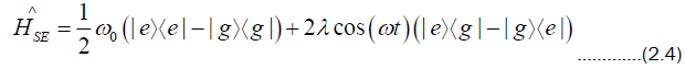
Even though this has been setup in a semiclassical way, the structure of the terms (2.4) is of the form mentioned for a two-state system decohering with a bath.
Interaction with quantized field
The field is now introduced so it is treated as quantized in the atom-field part of the interaction Hamiltonian and has the form,
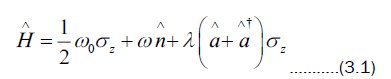
and  are the annihilation and creation operators for the quantized field respectively. They satisfy the
commutation relation
are the annihilation and creation operators for the quantized field respectively. They satisfy the
commutation relation 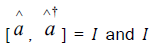 represents the identity operator. The operator
 is a number operator. When
 the system is on resonance, and if we work in the interaction picture, (3.1) leads to a Jaynes Cummings Hamiltonian given in terms of Pauli matrices as
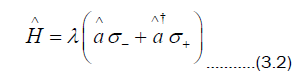
To study (3.2), we write Hamiltonian (3.2) using the following pair of operators defined to be
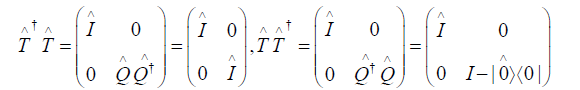
The two operators  in (3.3) satisfy the following two relations
This amounts to saying 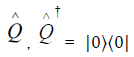 so from (3.3) writing
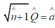 and defining the operator in terms of
 to be
to be
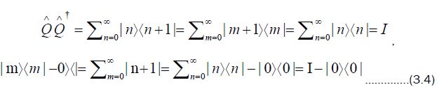
Using (3.5), we calculate that
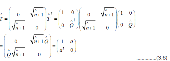
This implies that  in (3.2) can be written as
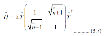
Also from (3.4) the operators  do not commute
The evolution operator can be determined from  by working out
  starting from (3.7). Proceeding inductively for �� ≥ 1, we have
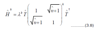
The operator  can be calculated using (3.8) as follows
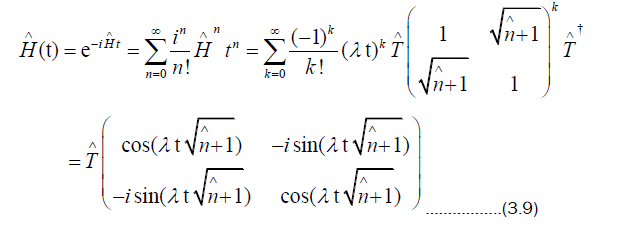
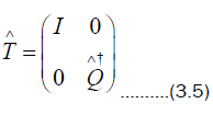
It suffices to write evolution operator  as
as
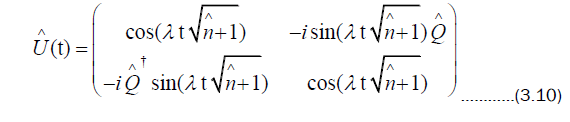
If a given initial atom-field state is postulated, by applying the evolution operator to it, the evolution of the system can be determined. Let the initial state have the product form
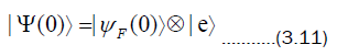
The field is in an arbitrary field state  and the atom is prepared in the state
 and so

As mentioned already, after the interaction part of the Hamiltonian has acted, the atom and field become entangled
in such a way that in general the wave function cannot be written in a form that is a multiplication of two distinct wavefunctions that relate back to the atom and field. However, due to the oscillatory nature of there will be times when the atom and field are also disentangled, or possibly completely so.
One way to study this is by means of atomic inversion, but other variables such as entropy can also be studied. The atomic inversion can be calculated using wavefunction (3.12) by using
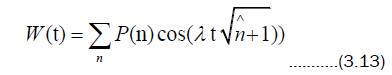
Here  is the photon distribution for state
  For example, one particular choice is
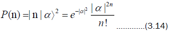
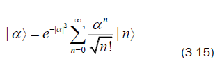
for a coherent state of amplitude  an eigenstate of the number state,
The atomic inversion can be studied numerically and the oscillations collapse so no oscillations occur for some period of time. Subsequently the oscillations revive. Such phenomena occur because of the constructive or destructive interference of the cosines in W(t). Although it appears like there is no more interaction in the collapse region, this is not so as the atom and field are exchanging phase information as they are strongly entangled. This will cause a quasi-entanglement at 1/2 the revival time. Then atom and field pass to quasi-super positions of excited, ground state and coherent states respectively.
The revival in the case of the super positions of coherent states are faster as neighbor terms that interfere constructively in (3.13) are separated. For a thermal distribution, neither collapses nor revivals occur. The cosine terms do not interfere constructively or destructively. Atomic inversions can indicate the state of the field.
Evolution of the density matrix
In the context of an open system, the master equation is a first order differential equation for the reduced operator of the system. The equation incorporates all the properties of the system reservoir dynamics, so knowledge of the initial density matrix and the ability to solve it permits the density operator to be given at any time.
There is an approach to the study of a dissipative cavity by means of the correspondence principle in the zero temperature limit. The evolution equation can be solved for several initial conditions such as coherent states, which keep coherent structure through dissipation, number states and states which are rapidly killed by the dissipation process. This equation can be generalized to the non-zero temperature regime and solved as well.
The solutions of the equation are based on the algebra satisfied by the operators that compose it. This can be done by disentangling the exponential of the sum of these operators. This is deeply linked to the solvability of the algebra.
There are many ways of developing this equation, for example, by invoking the correspondence principle. We just
concentrate simply on how it can be solved. Equations of motion valid for classical states, where coherent states can be thought of as quasi-classical, turns out to be valid for quantum states. A way to study the evolution of is by means of a master or Lindblad equation [2] which has the general structure,
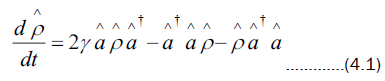
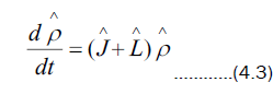
It is solved here for an initial coherent state so decay of coherent states can be studied. A general procedure can be introduced and developed for solving this kind of equation. Define the following two operators
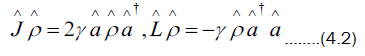
Differential equation (4.1) is given by
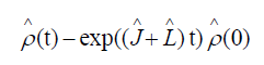
The solution to (4.2) has the general exponential form
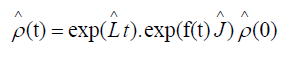
To factorize this exponential of operators, take an ansatz of the for
Differentiate both sides of  with respect to time
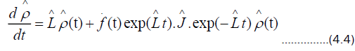
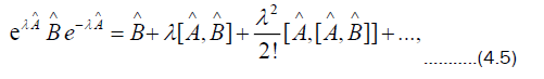
The derivative  with respect to t of f(t) appears in (4.4). To simplify (4.4), the Campbell Baker-Hausdorff
identity is used, and it is given by and it is given by and it is given by and it is given by
with respect to t of f(t) appears in (4.4). To simplify (4.4), the Campbell Baker-Hausdorff
identity is used, and it is given by and it is given by and it is given by and it is given by
It is necessary to compute the commutation relation  and the details are shown to provide an example
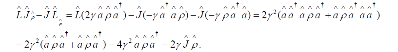
Consequently, the case with n= 1 commutator is proved: 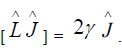 By means of induction on n, the typical commutator which occurs in the Baker-Campbell-Hausdorff formula where operator
  appears n times is
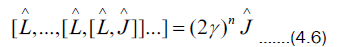
Taking 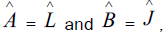 it follows that
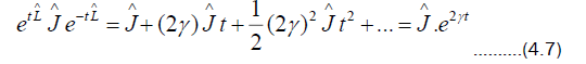
Substituting (4.7) into (4.4), it takes the form
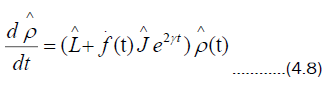
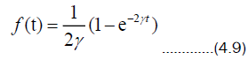
Comparing (4.8) and (4.3) it follows that function fis a solution to the initial value problem,
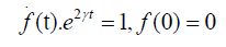
This problem has the following solution
With function (4.9), a solution to (4.1) is known, and it can be applied to any state. For example, for an initial coherent state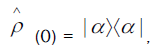 so expanding the second exponential in power series and applying
 to the density matrix of the coherent state we get

Coherent states are eigenstates of the annihilation operator. Apply the operator  to the coherent density matrix, then us
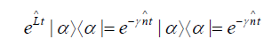
we finally obtain
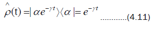
So for large  evolves to the state
 It may be conjectured that amplification can happen when
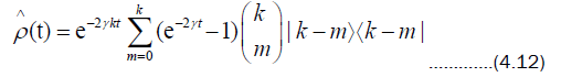
For an initial number state  the t-evolved density matrix is given by
If there exists a pure state  originally, then the decay takes it to a statistical mixture of number states and the vacuum is attained as
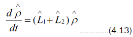
The differential equation for the operator  in a frame rotating at field frequency ��, which accounts for cavity losses at non-zero temperature under Born-Markov approximation is
If  is the average number of photons, then

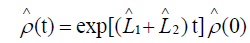
The formal solution to (4.13) has the same form as in the first problem
Now redefine the operators 

These operators obey the commutation relations 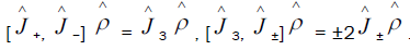 For example,

Analogous to the previous case, the solution to (4.13) may then be written
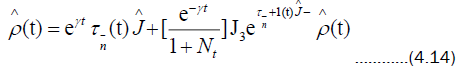
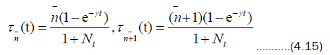
The following two functions appear in (4.14) with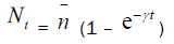
The steady state of  for any initial state of the field is the thermal state.
Entropy pure states and statistical mixtures
The interaction of a system with an environment results in the situation that the system looses its parity and develops then on into a statistical mixture. This degree or extent of mixedness can be examined by looking at the entropy and something else called purity, which are two closely related concepts. The relationship between decoherence and entropy creation has been of interest since the late 1980s. This is also related to processes such as energy redistribution and entanglement production [8-13].
Entropy is an important concept with which pure states or statistical mixtures can be distinguished. The quantum mechanical entropy is defined to be
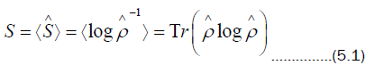
The quantity �� in (5.1) is called the von Neumann entropy and the Boltzmann constant has been set equal to one. If
the density matrix refers to a pure state, then �� = 0 in (5.1), and if it describes a mixed state, then �� > 0. It can
be said that S measures the deviation of the state from that of a pure state. A non-zero entropy accounts for additional uncertainties above the inherent quantum uncertainties that already exist. The density matrix of the system evolves in time by means of a unitary time evolution operator so its eigenvalues must remain constant.
The trace of an operator depends only on the eigenvalues of the operator which implies the entropy of a closed
system is time independent.
of the system evolves in time by means of a unitary time evolution operator so its eigenvalues must remain constant.
The trace of an operator depends only on the eigenvalues of the operator which implies the entropy of a closed
system is time independent.
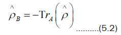
As systems tend to be coupled to other systems usually we do not have closed systems. The case of interest here, the interaction of an atom with a field or more generally with an environment was looked at already here. Consider a larger system composed of two-subsystems, such as atom and field. Although the entropy of the entire system remains time-independent, there is the question of what happens to the entropy of each subsystem. Suppose the two subsystems are called A and B, then the trace of the total density matrix over the basis of subsystem A produces the density matrix which refers to B and this is written as
Tracing over subsystem B gives the density matrix for A,
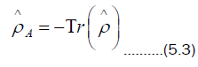
Using (5.2) and (5.3), the entropies for A and B may be defined as
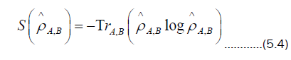
The effect of tracing over one of the subsystems means that each subsystem is no longer ruled by a unitary time evolution. This implies the entropy of each subsystem becomes time-dependent. Thus it may now evolve from a pure state to a mixed state, or from mixed to pure.
The following inequality for two interacting subsystems has been put forward by Lieb and Araki, which is
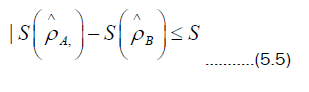
If the two subsystems are initially in a pure state, the entropy S = 0 and (5.5) yields that 
Another variable to classify states is called the purity parameter
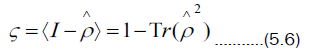
By using the eigenbasis of the density matrix, it is the case that
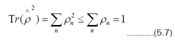
Equality holds for pure states, so this parameter differentiates between mixed and pure states. This leads to the
determination of a lower bound for the entropy S. Since in general 

Let us see how these concepts can be applied to the case of the atom-field interaction. Suppose both of these are initially in pure states, then either the atomic entropy or the field entropy can be studied and have to be equivalent by the Araki-Lieb theorem. Let us consider the atomic entropy, which requires us to write the atom density operator for the initial coherent state and atom in its excited state
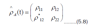
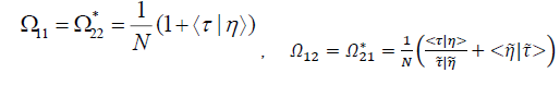
In (5.8), ρ22 = 1 − ρ11 and the matrix elements are given as
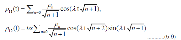
Let us set  to be the photon distribution for a coherent state. The eigenvalue of
 in (5.8) can be found by means of a secular polynomial which arises from the determinant of
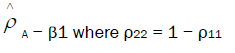
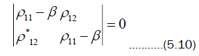
The secular polynomial is a quadratic and has the form,
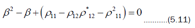
The solutions of this quadratic are the eigenvalues of (5.8) which we call β1 and β2. In terms of β1,2, the entropy S can be calculated from these as
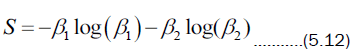
Therefore, we conclude that the atom and field get close to pure states at half the revival time when both functions are close to zero.
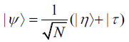
It is useful to conclude with a more serious example to illustrate this. Let  be a superposition of two coherent states
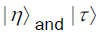 Normalizing this state by means of the quantity N,
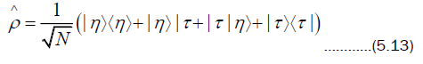
The density matrix corresponding to this state is
where 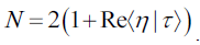 The solution to (4.4) similar to (4.10) for
 give
give
Setting 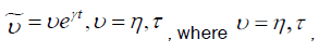 the density matrix must b
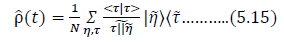
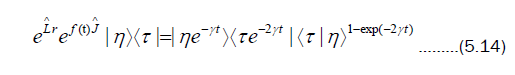
This implies that the density matrix evolves from a pure state to a statistical mixture. Density matrix (5.13) has a corresponding eigenvalue problem associated with it
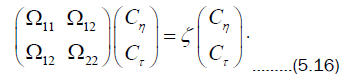
The matrix elements appearing in (5.16) are
The secular polynomial is again quadratic as it should for a two by two problem

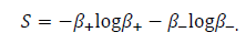
This produces two distinct eigenvalues in general, β±, from which the entropy is calculated as in (5.12)
Two level problems
A fundamental building element of quantum mechanics is the two level system. Although it is in principle possible for an atomic system to have only two bound states, there would usually be a continuum of unbound states or scattering states. In the ideal two level atom these continuum states do not exist.
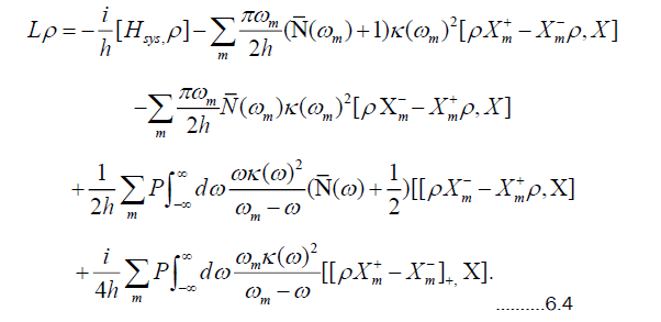
Considered more generally and abstractly as in (4.2), the master equation can be stated as
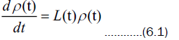
where L(t) is a linear operator whose form depends on the particular master equation. The operator in (6.1) may or
may not have an explicit time dependence. It is the intention here to present two cases of (6.1) and then use the
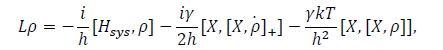
second one to study the evolution of the expectation values of a particular operator. If none of the terms in the Hamiltonian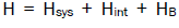 has any explicit time dependence, then neither will there be any explicit time dependence in L(t) if this is the relevant operator for evolution in the Schrodinger picture. For the case of quantum Brownian motion, it is the case that
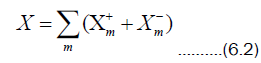
The operator X may be broken down into a sum of operators
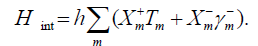
In the Schrodinger picture Hint can be written in terms of these as
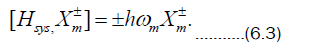
The eigenoperators of the system Hamiltonian just introduced obey the equation
This form is quite general since any system operator can be decomposed into eigenoperators of Hsys. For the quantum optical case of interest here
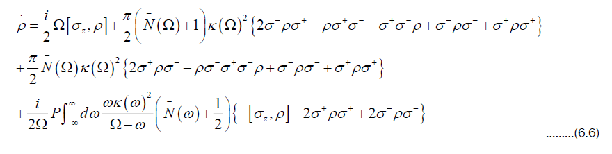
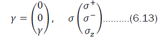
Let us just consider the optical case and look at a two level atom in an electromagnetic field. Then in this case, operator X is taken as

This corresponds to splitting up X into eigenoperators so that m takes only one value. Using the Pauli algebra

the matrix equation can be reduced to
The master equation for  combined with the cyclic property of the trace operation and Pauli matrix algebra (6.5) can be used to obtain evolution equations for the means of the operators σ± and σz by means of
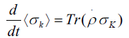
Start with the case k=z and multiply both sides of  and then take the trace
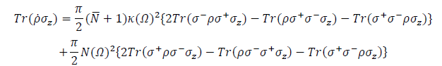
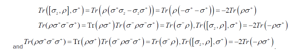
Using the algebraic relations (6.5), the traces here can be simplified
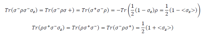
Similarly in the second term, we find that
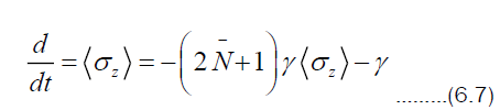
If we set  then the evolution equation takes the form,
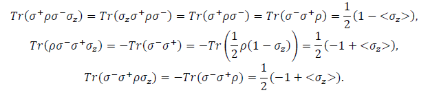
The evolutions or rates of change of the quantities  can be calculated in a similar way. Putting
and as well using
 Substituting these results into the equation for
 we find that

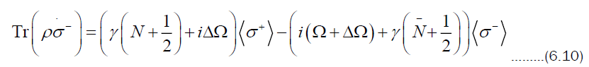
Finally using  and
and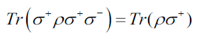 it is found that
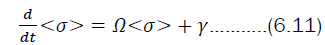
These results can be summarized in matrix form,
where the matrix variables in (6.11) are given by
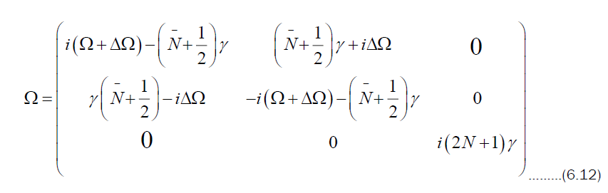
and
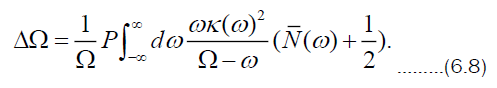
From the structure of matrix Ω in (6.12), ΔΩ represents a frequency shift in the sense that it occurs in ρ as the coefficient of a term [σz, ρ] which is of the same kind as the original system Hamiltonian. In the interaction with the bath or radiation field in this case, the frequency observed is term is finite for
 and vanishes when T = 0. This yields a shift caused by the thermal radiation which the atom experiences and is connected with the Stark shift. The Lamb shift would be related to the part proportional to the 1/2 and has its source in vacuum fluctuations.
It has been seen that system-reservoir coupling has the consequence that quantum coherence decays, that is, through the process of decoherence. Some approaches have been considered, however, a powerful way to approach this is to consider an evolution equation called a master equation. A master equation has been studied here for different quantum systems which come up for example in real optical systems. As a general statement it can be said the interaction of the quantum system with a reservoir means that the quantum coherence effectively decays. Dissipation quickly kills off coherence taking an initial pure state to a statistical mixture of states. It is possible nonetheless to learn a lot with regard to the quantum field in a cavity in spite of dissipation. By solving such an equation, a way can be found that permits the study of for example the quantum state of light. This should have an impact on the practical problem of transmitting optical signals carrying information by means of optical cables.
[Crossref] [Google Scholar]
[Crossref] [Google Scholar]
[Crossref] [Google Scholar]