Fractional Time Defect-Diffusion Model of Dielectric Relaxation

Abstract

The defect-diffusion model has been used to explicate dielectric relaxation and other relaxation phenomena observed in some dielectric materials. In the model it was assumed that the defects move through the system by random-walk in one-dimension and the relaxation, which is instantaneous and independent of the state of other dipole sites, can only occur when a defect diffuses to a dipole. In this study, the defect-diffusion model is reconsidered by using the fractional calculus technique, and the model is extended to one- and three-dimensional fractional defect-diffusion model. A dipole correlation function derived from the fractional approach is identical with the Kohlrausch-Williams-Watts (KWW) non- exponential relaxation function, which is universal for describing the relaxation data of a wide variety of polar materials. Then, a new fractional complex susceptibility obtained from the defect diffusion model assisted fractional calculus is exposed, and it is shown that the results are compatible with empirical Cole-Cole and the Cole-Davidson type behavior, and Havriliak-Negami behavior is also obtained under the certain limits. The results obtained lead to a molecular interpretation of non-Debye type behavior. This suggests possible microscopic mechanisms for relaxation in polar materials having molecular chains.

Keywords

Dielectric relaxation; Defect diffusion; Fractional calculus; Fractional time

Introduction

In the dielectric relaxation theory, the frequency dependent dielectric constant is given as

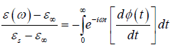(1.1)

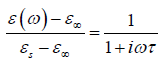
where ε_∞ is the high-frequency limit of the dielectric constant and εs is the static dielectric constant [1]. The function φ(t) describes the decay of polarization of a dielectric sample with time after sudden removal of a steady polarizing electric field. In Debye's classical theory [2-4] of dielectric relaxation, φ(t) is postulated to be a decaying exponential given by.

(1.2)

where τ is the temperature-dependent relaxation time characterizing the Debye process. Then the relation function as first obtained by Debye is true for the frequency domain:

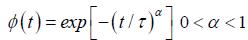
Although experimental dielectric relaxation data obtained from many materials composed of simple molecules compatible with the Debye model, important deviations appear in many complex materials, which includes e.g., glasses, disordered crystals, supercooled liquids, amorphous semiconductors and insulators, polymers and molecular solid solutions [5]. It has been shown that the dielectric response of such different complex physical systems is characterized well enough by KWW function [6] in the time domain:

(1.3)

For α=1 the KWW function becomes the Debye function. Moreover, many investigators have found that the KWW function represents a universal model for a wide class of materials, especially polymeric substances and glasses. The great empirical success of the KWW relaxation function has motivated the scientist to seek physical models to give a meaning to it.

The purpose of this paper is to examine the nature of the fractional KWW function obtained by using the fractional approach and introduce such a new model based on the fractional calculus, namely fractional defect diffusion model.

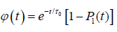
Glarum [7] proposed a defect diffusion model of the dielectric relaxation processes in amorphous materials. In this model, it was assumed that the defects move through the system by random-walk in one-dimension and relaxation, which is instantaneous and independent of the state of other dipole sites, can only occur when a defect diffuses to the dipole. In this model the dipole correlation function is given by

(1.4)

where τ0 is the relaxation time of molecular orientation without defects around the dipole, and P₁(t) is the probability for a molecule to be reached by a defect within a time interval t. The motion of the defect is given by the continuum diffusion equation

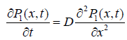(1.5)

where D is the diffusion coefficient of the defect. Under some conditions Glarum reached to the dipole correlation function as

(1.6)

for the one dimensional nearest neighbor defect diffusion process, where τ_D is Afterwards, many authors have attempted to develop Glarum’s model by incorporating the more than one nearest defect in order to eliminate the anomaly of the dipole correlation function derived first from Glarum’s model. Moreover, [8] have attempted a three-dimensional analysis of the defectdiffusion model, so that this would eliminate the need to introduce the second nearest defect process is considered by Philips et al.[9]. Hund and Powles’s analysis has shown that the extension of the one dimensional analysis to three dimensions does not substantially alter the satisfactory conclusions of the one dimensional analysis. Bordewijk [10] improved the defect diffusion calculation by considering a relaxation from all defects, not only just the one that is nearest by, and found a relaxation function of the KWW [11,12] with the exponent (α=1) in one dimension and the Debye relaxation α=1 in three dimensions, but also we know that most glass forming liquids and amorphous polymers exhibit strong deviations from the Debye relaxation function. Skinner [13] has developed a relaxation model for polymers based on both kinetic Ising model of Glauber [14] and Bordewijk’s defect diffusion model. Correlation function obtained from their model are well represented by the KWW relaxation function with 1/2<α<3/4. Bozdemir [15] has generalized the model by introducing a new one dimensional molecular chain defect diffusion model. He assumed the defect distributions to be in the form of Gamma-density function with non-integer powers, and the relaxed unit as being a linear chain molecule having defects, time- delayed molecular-correlation function obtained is in the form of KWW decay function with 0<α<1.

In this article, it will be demonstrated that a physically acceptable analysis of a new one- and three dimensional fractional defect-diffusion models are possible, by using the fractional calculus technique, if one considers the fact that the relaxing unit is not only an individual dipole itself associated with a chain, but the chain as a whole [15]. As will be shown from the analysis of this new version of the defect-diffusion model, a number of physically important results can be obtained, such as KWW relaxation function, empirical Cole-Cole [16] and Cole-Davidson [17] type behavior, and also Havriliak-Negami [18] dispersion relation.

Fractional Integrals and Derivatives

In this study defect diffusion model is reconsidered in terms of fractional time in one- and three-dimensions by using the fractional calculus technique. Many definitions, which include Riemann-Liouville, Weyl, Reize, Campos, Caputo, and Nishimoto fractional operator, have been proposed about in the last two centuries. The most widely used definition of an integral of fractional order is by means of an integral transform namely the Riemann–Liouville integral. According to the Riemann–Liouville approach, the fractional integral of order is defined as

(2.1)

For α > 0, t > 0. Moreover, if U(t) is continuous for t ≥ a, fractional integration has the following property

(2.2)

Furthermore, under certain assumption

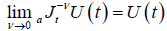(2.3)

so it can be written

(2.4)

One of the most important properties of the Riemann-Liouville fractional approach is that

(2.5)

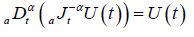
The Riemann-Liouville fractional differentiation operator is a left inverse to Riemann-Liouville fractional integration operator of the same order . Where is Riemann-Liouville fractional derivative and defined as

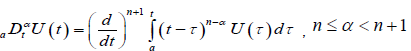(2.6)

More details and properties of the fractional operator Jα and Dα can be found in [19-21].

Fractional Evaluation Of The Defect Diffusion Model

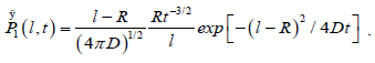
The essential feature of the defect diffusion model is that there is a cooperative interaction between the relaxing dipole and its nearest-neighbors containing defects, and the relaxation can only emerge when a defect interacts with a dipole. The probability P₁(l,t) for a defect at a distance l from a molecule to arrive at the molecule within the time interval t is given by Chandrasekhar’s result [22] for diffusion in the presence of an absorbing wall:

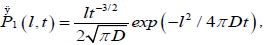(3.1)

where D is the diffusion coefficient appropriate to the motion of the defect in the material. Firstly, if we assume that dipoledefect interaction process is a nonlinear function of the time we can suppose that the irregularity in the flow of the time determines the form of the probabilities, which should be a part of the fractional space in which the orientation of the molecules takes place. In this view, the probability P₁(t) is obtained by averaging P₁(l,t) over all possible values of l by using the probability density of the spatial separation of defects given by f(x)=1/a, which is in agreement with Bordewijk’result.

We suggest that the transition probability per unit time for the nearest defect to reach the dipole for the first time can be evaluated using the fractional time integral. In this way, using the Riemann-Liouville fractional integral to evaluate the probability transitions, we can write

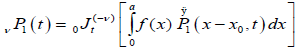
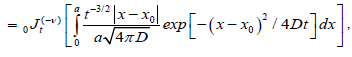(3.2)

where is the Riemann-Liouville fractional operator given by equation (2.1). So, under the assumption that the media have macroscopic dimensions, x0 and a-x0 are large for representative molecule, we reach to fractional probability

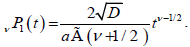(3.3)

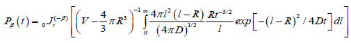
Suppose we have a dipolar chain with N defects and define P₁(t) as the probability for a dipole to be relaxed within a time interval t by a single defect after the external field has been turned off. Similarly, P(t) is defined to be the probability for the whole chain to be relaxed at time t by any of these defects. Accordingly, the probability for a dipole not to be relaxed by a defect is given by 1-P(t), while the probability 1-P(t) for the whole chain not to be relaxed by any of these defects is given by

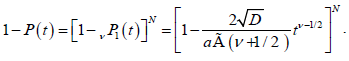(3.4)

Taking the limit of the equation (3.4) for N→∞, substituting a=2Nl₀, we reach to

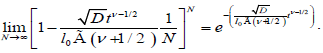(3.5)

If the relaxation time τ is selected in the forming of 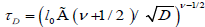, we obtain a one-dimensional fractional correlation function as

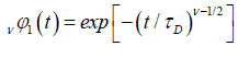(3.6)

which is a KWW-type function. As expected, for v=1 the equation is compatible with the Bordewijk’s result in one-dimension. It is noted that this fractional decay function tends to zero as t→∞ and describes the region left between Cole-Cole and Cole- Davidson behavior in the dielectrics. Dielectric relaxation data of a variety of amorphous polymers have been well described by this function, finding that 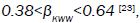but for fractional approach 0.88<V<1 is meaningful.

In the three-dimensions, in agreement with Hunt and Powles [8], the probability of a defect at a distance l from a molecule to enter a sphere with radius R around the molecule within a time interval t is given by

(3.7)

Excluding the sphere with radius R, and by using fractional approach to the problem, as for the one-dimensional case, we can write the probability depended on the fractional time exponent

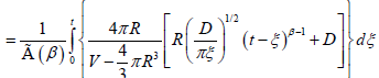
(3.8)

Hence, for and where d0 is the density of defects, the change for a molecule not to be reoriented by a defect located at an arbitrary position can be written as, for N defect,

(3.9)

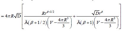
So, taking the limit of equation (3.9) for N?8, we obtain the fractional time dipole correlation function in tree-dimensions

(3.10)

where 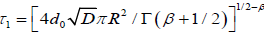and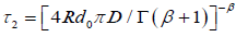 . Equation (3.10) has two part of the defect diffusion:

In this concept, we can say that 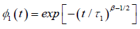represents the one–dimensional correlation function of the molecular chain, identical with the equation (3.6), and 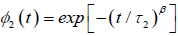represents the relaxation of a single dipole with respect to the molecular chain. The data obtained by many workers studying relaxation in different systems are fitted well by where are KWW’s constant. In our one dimensional fractional case, the fractional β parameter is found to be in between 0.86 and 0.92, so exponent ranges which is quite compatible with the values obtained from the experimental results. Moreover, in certain polymeric materials, larger values for β have been also observed such as in polyvinylacetate, where the KWW exponent is 0.56. So that, even if polymeric materials are in a certain sense one dimensional, there must have some components, directing in a different way affecting the relaxation substantially. In this context, we can say that interactions of the charged particles with each other and also with defects at different speeds lead to a distribution of relaxation times. Even if some attempts made by using the relaxation time distribution functions to explain this situation, this approaches has been subject to criticism by Jonscher [5] due to the absence of its physical meaning.

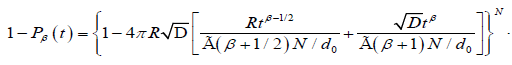
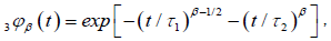
We show that the behavior of the defect diffusion part of the correlation function depends on the τ₁ and τ₂ relaxation times. So, in the case of R is extremely small, τ₁ >> τ₂, we obtain an exact KWW function

where We show that, from the equation (3.6) and (3.10), for a given v and β in φ(t), the rate of finding in one dimension is less than three dimensions. At this point we can say that the finding probability of a dipole by a defect shrinks with decreasing R in accordance with the mathematical and physical structure. Large R values reveal a one-dimensional situation, which is compatible with the other investigator's result mentioned at the beginning of the article.

Fractional Model Of The Defect Diffusion

If it is assumed that the relaxing unit is not only an individual dipole itself associated with a chain, but the chain as a whole, and the probability density of the nearest neighbor defect located between l + dl exhibits the a normal distribution [25]

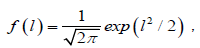(4.1)

we can write for the P(t), which is the probability per unit time that a defect arrives at the point l=0 for the first time at t > 0,

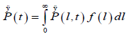
(4.2)

Integrating the result (4.2) with respect to t gives

(4.3)

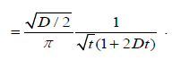
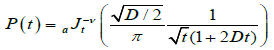
where D=1/2D. From this relation, we obtain the correlation function of the dipole orientation as

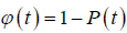
(4.4)

for the nearest defect diffusion process. A graph of correlation function versus log (t) is shown in Figure 1.

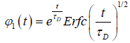
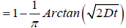
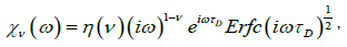
Thus, we reach to the complex susceptibility as

(4.5)

where Erfc(.)is the complementary error function [26]

(4.6)

So, for τ_D=1/2D the complex susceptibility can be written as

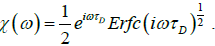(4.7)

A plot of loss factor x” (ω) versus log (wτ_D) is shown in Figure 2. As expected, the variation of the diffusion coefficient D changes the relaxation time, and this situation also leads to a slip of the frequency peak from low frequency to high frequency. Figure 2 shows that equation (4.7) exhibits the Cole-Cole behavior.

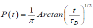
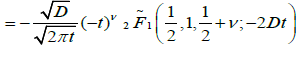
It is assumed that the probability has a fractional form in the time space, dipole-defect interaction process is a nonlinear function of time, namely, irregularity in the flow of the time determines the form of the probabilities. In this view, let P(t) be the transition probability that a defect arrives for the first time during the time interval t at the point x=0 can be evaluated by using the fractional time integral. In this way, using the Riemann-Liouville fractional integral operator (2.1) to evaluate the probability transitions, we reach to

(4.8)

where is the regularized Gauss hypergeometric function defined by

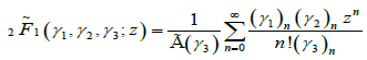
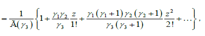(4.9)

Where 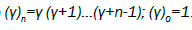Also, using the relation in the equation (3.5) we can obtain the complex susceptibility as

(4.10)

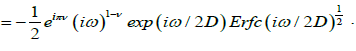
Thus, for τ_D=1/2D a new fractional complex susceptibility is written as

(4.11)

Where A plot of loss factor x”(ω) versus log(τ_D) is shown in Figure 3.

So that, we have been experienced a result obtained from the structure of the fractional time stochastic diffusion process. In the system under consideration, there might be some combinations of diffusion processes which have different values of this internal time scale, and they might also be affected differently by the disorder in the system. Such a situation could more accurately be addressed with a fractional view for a cooperative dipole-defect relaxation mechanism. We can suppose that different mechanisms involving the relaxation are an average function of the relaxation process, and it can be said that this situation causes to exhibit an average fractional time on the whole time domain.

Conclusion and Discussion

We know that many various relaxation phenomena in the nature comply with the fractional power laws in time and frequency domains. Fractional time evolutions to relaxations indicate that the probable source of these processes lies in the nature of chaotic phenomena, and that fractional powers of the time is an essential conclusion of the stochastic construction of the relaxation processes [27]. So, we may say that the behavior of the relaxation processes shows that the fractal structure of the nature, including the stochastic processes works in the fractional time. This perspective compels us to use the fractional theory on the relaxation processes. In this paper, the exact KWW function is obtained by using such a fractional approach on the dielectric relaxation based on the defect-diffusion model, which is universal for describing the relaxation data of a wide variety of polar materials.

Moreover, under the suggestion that the relaxing object is not only an individual dipole, but a dipolar chain having a number of defects such as a polymer chain. In this context, it is clear that the response function is an average function of the fractional time. So, we are calculating another independent relaxation processes which could be the relaxation of a site in the absence of a defect. In the system under consideration, there might be combinations of diffusion processes which have a different value for this internal time scale, and they might also be affected differently by the disorders in the system, i.e., exhibit a different power law in the time domain. Therefore, the combined relaxation process might be composed of two or more individual interactions, which causes to more elaborate relaxation forms. On the other hand, the nearest neighbor interactions between particles have not the same time intervals and velocities because of the time is fractionally changing, namely, in the microscopic levels (or electronic) the flow of the time is quantized. This situation makes it necessary to develop a new fractional statistics. At the same time we may say that the fractional β value, which shows a degree of movement of the defects, should be dependent on temperature and pressure; 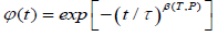and β values around the 0.5 compatible with the experiment makes sense to use the Normal distribution.

In conclusion, we have introduced a connection between relaxation processes and fractional dynamics for the non-Debye type behavior, where it can be assumed that the defects have a fractional normal distribution in the time space of the probability, this situation arrives us to fractional complex susceptibility exhibiting the same characteristics with the Cole-Cole, Cole-Davidson and Havriliak-Negami behavior while the fractional exponent v changes from V=0.6 to V=1 (Figure 3). At this point, we can say that this situation is resulted from the fractional nature primarily responsible for determining the form of loss curves observed in a variety of polymers and other substances having dipolar chains.

References

1. Shlesingert MF andMontrollt EW. On the Williams-Watts function of dielectric relaxation. Proc. Natl. Acad. Sci. 1984;81:1280-1283.
2. Bottcher CJF andBordewijk P. Theory of Electric Polarization. Elsevier.1992;2.
3. Frohlich H. Theory of Dielectrics, Clarendon Press, Oxford. 1958.
4. Hill NE, et al.DielectricProperties and Molecular Behavior. Van Nostrand, London. 1969.
5. Jonscher AK. Universal Relaxation Law, Chelsea Dielectrics Press, London. 1996.
6. Williams G, et al. Further considerations of non symmetrical dielectric relaxation behaviour arising from a simple empirical decay function. Transactions of the Faraday Society. 1971;67:1323–1335.
7. Glarum SH. Dielectric Relaxation of Isoamyl Bromide. J. Chem. Phys.1960;33:639-643.
8. Hunt BI andPowles JG.Nuclear spin relaxation and a model for molecular reorientation in supercooled liquids and glasses. Proc. Phys. Soc.1966;88:513-528.
9. Phillips MC, et al. Relaxation in Liquids: A Defect-Diffusion Model of Viscoelasticity. Proc. R. Soc. A 1972;329:193-218.
10. BordewijkP. Defect-diffusion models of dielectric relaxation. Chem. Phys. Lett.1975;32:592-596.
11. Cardona M, et al. The history of the stretched exponential function. Ann. Phys. (Leipzig). 2007;16:842-845.
12. Milovanov AV, et al. Stretched-exponential decay functions from a self-consistent model of dielectric relaxation. Physics Letters A. 2008;372;2148-2154.
13. Skinner JL. Kinetic Ising model for polymer dynamics: Applications to dielectric relaxation and dynamic depolarized light scattering. J. Chem. Phys. 1983;79:1955-1965.
14. Glauber RJ.Time‐Dependent Statistics of the Ising Model. Journal of Mathematical Physics. 1963;4:294–307.
15. Bozdemir S. Some comments and corrections on the defect diffusion models of dielectric. 1985.
16. Cole KS and Cole RN. Dispersion and Absorption in Dielectrics I. Alternating Current Characteristics. Journal of Chemical Physics. 1941;9:341-352.
17. Davidson DW and Cole RH. Dielectric Relaxation in Glycerol, Propylene Glycol, and n‐Propanol The Journal of Chemical Physics. 1951;19:1484–1490.
18. Havriliak S and Negami S. A complex plane analysis of α-dispersions in some polymer systems. Journal Polymer Science (Part C: Polymer Symposia). 1966;14:99–117.
19. Miller KS and Ross B. An Introduction to the Fractional Calculus and Fractional Differential Equations, John Wiley and Sons Inc, New York.1993.
20. Oldham KB andSpanier J. The Fractional Calculus, Academic Press, New York.1974.
21. Podlubny I. Fractional Differential Equations, Academic Press, New York. 1999.
22. Chandrasekhar S. Stochastic Problems in Physics and Astronomy, Reviews of Modern Physics. 1943;15:1-89.
23. Williams G. Molecular aspects of multiple dielectric relaxation processes in solid polymers, Advances in Polymer Science. 1979;33:59-92.
24. Phillips JC. Microscopic theory of the Kohlrausch relaxation constant . Journal of Non-Crystalline Solids. 1994;172-174.
25. Jagdish KP, et al. Handbook Of The Normal Distribution, CRC Press, New York.1996.
26. Yudell LL. The Special Functions and Their Approximations, Academic Press, London.1969.
27. Relaxation. Physica Status Solidi (b).128:119–131.