Research & Reviews: Journal of Ecology and Environmental Sciences
ISSN: 2347-7830
ISSN: 2347-7830
1Leibniz-Centre for Agricultural Landscape Research, Institute of Landscape Systems Analysis, Eberswalder Str. 84, 15374 Muencheberg, Germany
2Leibniz-Institute of Freshwater Ecology and Inland Fisheries, Mueggelseedamm 310, 12587 Berlin.
3Leibniz-Institute of Freshwater Ecology and Inland Fisheries, Alte Fischerhuette 2, OT Neuglobsow 16775 Stechlin.
Visit for more related articles at Research & Reviews: Journal of Ecology and Environmental Sciences
A concept is rendered to replace the right-hand side of a set of ordinary differential equations with fuzzy models. This modeling approach allows stake- holder/expert knowledge to be included in the model development, leading to a white box approach and high credibility of models. An additional effect is that models are simple and stable. The system behavior can be controlled flexibly by fuzzy models; a number of examples are presented in the paper. Stability is investigated using the Lyapunov exponent. The approach is demonstrated using a simple aquatic ecosystem model and supported by open source software, namely the “Spatial Analysis and Modeling Tool” (SAMT), with additional modules written in Python.
Ordinary differential equation (ODE), Fuzzy modeling, Nonlinear systems, Dynamic fuzzy simulation, Simulation, Stakeholder-based approach, SAMT, Python.
Mathematical modeling is an important instrument for investigating complex relations in our human world [1]. Mathematical modeling is extremely useful not only in economics, but also in technical and science disciplines. Three main pillars that explain why mathematical modeling is important can be identified: simulation/prognosis, decision support and understanding.
Simulation/prognosis: Models and simulation in environmental sciences are often applied to investigate possible ecological states in the future or to simulate situations that are virtually impossible to realize experimentally or that cannot be performed for ethical reasons, and so on. Examples of this type of simulation are
• modeling the movement of species as shown in [2-3],
• Change to a landscape caused by extreme weather conditions [4]
• A biochemical model in an aquatic system [5] and
• Ecosystem models
– such as SALMO [6] DELAQUA [7] and
– DYRESM-CAEDYM [8]
Just to mention a number of examples from the vast array of ecosystem models available (a relatively recent overview can be found [9]. A very rich source of models is the register of ecological models 1, the description of ECOBAS [10].(Ernst et al., 1997). For example EMMO [11] can be found there.
Decision Support: The use of models to provide a basis for decision making is growing in importance. SALMO, for example, was developed to help manage water reservoirs (see, for instance, the GETAS project)2. This class of modeling also includes statistical analysis, as shown in [12] models for transferring semantics to users, such as that discussed in [13], and so on. According to [14], the use of models to support decision-making should include stakeholders in the actual modeling process. This open modeling approach increases the credibility and level of acceptance of simulation results. It is also not necessarily less accurate than simulation models. It was shown in [15] that a simple model based on expert knowledge can generate better results than a highly sophisticated process oriented model.
Understanding: The mathematical model need not necessarily be complex in order to its interactions to be understood. It suffices if (simple) models do not seriously contradict experimental knowledge, i.e. if they de- scribe the observed phenomena qualitatively correctly. This type of model is known as minimal model [16] Scheffer has shown in numerous publications how such a type of model can help us to understand complex ecological interactions. The advantage of minimal models is that mathematical formulations are simple, and there is less need to find parameter values and to run models with default values.
Summarizing: Minimal models may be described as being “as complex as necessary but as simple as possible”. The general need in mathematical modeling is abstraction. It is evident that the degree of abstraction, i.e. the extent to which details are not mapped in a mathematical description, is a matter of actual knowledge and of the aim of modeling. The degree of abstraction even depends on the modelers taste and intuition. In [17] (page 9), a graphical model is shown visualizing the existence of an optimum: a more detailed mathematical model will produce a lower process-related bias at the cost of the uncertainty of measured input quantities, whereas a less detailed model will be biased with respect to the relevant processes. An acceptable compromise must be found. When statistical models are applied, the existence of an optimum can be directly shown, as demonstrated by [18].
In this paper, a proposal is made to replace the right-hand side (rhs) of Ordinary differential equations (ODE) with dynamic fuzzy systems. It will be shown that this fuzzy approach leads to an easily understandable and adaptable model. In addition, the model is highly flexible towards model functional behavior, and should exhibit good numerical stability. In the words of [14], the resulting modeling framework should be considered as “participatory modeling”, not only for stakeholders as in the mentioned publication, but also during a preceding stage for efficient cooperation with experts involved in conducting experiments.
A minimal model, following the ideas of Scheffer [19], contributes to the controversial ecological debate about the mesotrophic maximum hypothesis (MMH), which state that a low level of nutrition leads to a food web system with a few interactive paths. A high level of nutrition, i.e. eutrophic or hypertrophic systems, may lead to a complex food web with many interaction paths or to the absence of these very paths that transfer energy upwards to the top of the food web. Therefore the hypothesis is that in mesotrophic systems, the food web is rich enough to allow energy to be transferred from nutrition to top systems, but poor enough to be efficient. The basic model is schematically explained in (Figure 1).

Figure 1: Conceptual model as a basis for the minimal model “MMH”.
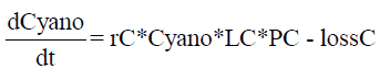
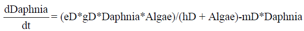
In a real lake ecosystem, the three selected groups – zooplankton (daphnia), edible algae (algae) and inedible algae (cyano) – are virtually always diverse communities comprising a variety of species. Thus, the presented scheme must be considered a strong simplification for the sake of indicating the potential of the modeling approach. The following system of ODEs describes the interactions shown in Figure 1, whereby the nutrition (soluble reactive phosphorus) is modeled as a parameter in the term P A (see equation1). Both algae and cyanos are described by a growing term (rX *Y *LX *P X ), where X is either C yano or Algae. Y stands for the population of C yano or Algae. Both C yano and Algae have a loss term (mortality, modeled after [20] and reduction by a flux term). LX describes the light influence, depending on water depth and the role played by blooms. In contrast to C yano, Algae are edible by species that, in a simplistic manner, are ascribed as belonging to zooplankton. A term analogous to gD* Daphnia * Algae/(Algae + hD) does not appear in the ODE for C yano because cyanos represent inedible algae
Finally, the ODE for Daphnia describes the increase in biomass from grazing (with efficiency, eD) and a loss by mortality (coefficient, mD).
 (1)
(1)
 (2)
(2)
 (3)
(3)
The idea is that, together with a description of the efficiency of energy transferred to Daphnia (trophical transfer efficiency, TTE), a maximum in the TTE can indeed be found if the parameter of nutrition is varied from low to high values [21].
We are aware that the model equation 1-3 is merely a simplistic approach compared to simulation models. Nevertheless, we prefer a simple model for this introductory text. A dynamic fuzzy model replaces the rhs of an ODE with a combination of fuzzy models. Fuzzy models can implement linear and nonlinear process descriptions, as shown by [22]. This means that fuzzy models can implement a nonlinear behavior, as shown in the original
model in terms such as gD∗Daphnia∗Algae/(Algae+hD), which is known as Monod kinetics [23], In addition to sigmoid Monod kinetics, fuzzy models are also capable of implementing more complicated interactions. The most important aspect is that biologists in the ecosystem modeling team, who are not necessarily familiar with the requirements of algebraic expressions of the rhs of ODEs, can infer knowledge in a broad sense, without knowing the ins and outs of the numerical consequences behind the model. In a “broad sense” means that knowledge about a system can be expressed in terms of rules that do not necessarily include only one single process (see below).
Fuzzy models are developed in four steps as follows:
• Definition of the membership function to fuzzify inputs,
• Definition of the outputs,
• Fill in the rule base as a combination of the membership function to the outputs,
• Check the model using graphical analysis.
The development of fuzzy models is supported by open source software, namely the Spatial Analysis and Modeling Tool (SAMT) [24], which has an integrated fuzzy toolbox. It is important to mention that checking the model is also a step in the model developing process, supported by the toolbox.
 (4)
(4)
 (5)
(5)
 (6)
(6)
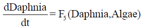
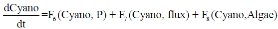
Equations 4-6 are derived from the additive structure of equations 1-3, whereby the loss terms are considered as parts of F1 and F6. Note that in the original equations (1-3) and in (4-6), phosphorus P is reduced to pf = P −(pgA*Algae+pgC ∗C yano) by Algae and C yano during the simulation; (pgA and pgC are constants). Compared to the original system, the interactions are now implemented more directly: for example, F1 (Algae, P ) expresses that an algae will uptake phosphorus and term F2(Algae, Daphnia) describes that algae will be grazed by Daphnia.
Nevertheless, fuzzy models are part of an ODE, as required for describing temporal evolution. This means that the result also depends on the simulation time and step size. The dynamic fuzzy simulator [25], which is now part of the open source software SAMT, was developed so that biologists would not require an additional tool. The dynamic fuzzy simulator [25] was developed and is now part of the open source soft- ware SAMT. In addition to carrying out general checks using SAMTs fuzzy toolbox, the fuzzy simulator enables the dynamic behavior to be checked, as well as the complete implementation of dynamic fuzzy models, including the graphical visualization of the systems behavior.
Model development requires three basic steps:
1. Implementation of fuzzy models
2. Implementation of the system of ODEs
3. Analysis of the dynamic behavior. These steps are described below.
The complete model including all fuzzy models, the ODE code and a visualization of the results can be found as open source code on the website3 . Without loss of generality, the model “algae daphnefis” (F2) is selected to explain the fuzzy approach. The basics of the fuzzy algorithm used are described in [26]. Model F2 describes the relation between Daphnia and Algae, implementing a predator-prey model [27]. Both state variables Algae Figure 2 and Daphnia (Figure 3) are inputs of membership functions; the ordinate is the degree of subsethood; and the abscissa is the concentration of the population considered (algae) (Figure 2).
If, for example, the relative concentration of Algae is 0.25, then it belongs to a degree of μmh(0.25) = 0.2 to the class “medium high” (mh) and with a degree of μm (0.25) = 0.8 to the class “medium” (m) (Figure 3).

Figure 2: Membership function input Algae є [0, 1].

Figure 3: Membership function input Daphnia.
For example, Daphnia belongs to the class medium (m) when (Daphnia = 0.2) is the value on the abscissa (μm(0.2) = 1.0) After defining the member- ship function of the inputs, modelers have to define the output function. So-called “singletons”, which can implement both nonlinear and linear models, are used as the output function [24]. Nonlinear systems have a much richer behavior and more interesting features than linear models [28].In particular, nonlinear models can express ecological knowledge much more easily than linear models are able to. On the other hand, there is no closed theory available for fuzzy systems, and modelers have to use Monte Carlo simulations as a tool for investigating nonlinear systems.
After establishing the set of membership functions for Algae and Daphnia (Figures 2 and 3), we have to clarify what the consequence could be for Algae, for example, with respect to the term F2 considered here. The possible outcomes arbitrarily span a range from [−0.02, 0] in an equidistant manner. We call the resulting system of discrete outcomes (according to the discrete number of combinations of Algae, Daphnia memberships) “singletons”, denoted by ni . The fuzzy model interpolates linearly between singletons to implement a smooth behavior (see, for instance, equation 7) (Figure 4).

Figure 4: Singletons as output.
The outcomes (n0 = 0.0, n1 = −0.005, n2 = −0.01, n3 = −0.015, n4 = −0.02) express that a high relative concentration of Daphnia will reduce the relative concentration of Algae.
The fuzzy model itself contains 5 * 6 rules corresponding to the combinations of membership functions of inputs with singletons. A selection of the rules is presented in (Table 1).

Table 1: Excerpt from the rule base of F2.
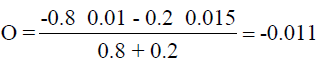
For example, Algae = 0.25 and Daphnia = 0.2 lead to a membership function for Algae μmh(0.25) = 0.2 and μm(0.25) = 0.8 (as shown in Figure 2); for Daphnia μm(0.2) = 1.0 (Figure 3). Therefore rules 15 and 21 willfire. Correspondingly, the final output O of the fuzzy model is (equation 7):
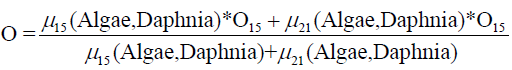 (7)
(7)
A complete description of the fuzzy algorithm can be found in [29].
The system of ODEs and the fuzzy models (the right-hand side of ODEs) define the simulation model. The simulation comprises the numeric to solve ODEs, simulation control (for example the number of iteration steps, step size, etc.), management of simulation parameters (initial states for system parameters, definition of control parameters such as phosphorus, flux) and visualization of the simulation results. The simulation system was implemented in the programming language Python. Python is an interpreter language developed by W. Rossum4 that is attracting a growing amount of interest. For example, Python is the scripting language of the leading GIS software AR- CGIS5 . The second author developed open source software for an ordinal analysis of data matrices, PyHasse, Here, Python is used together with its modules: ODE solver, the “odeint” of the Python library “SCIPY”6 , was used and “Matplotlib” for visualization7 The solver for the fuzzy module was written in C++ and wrapped in Python code using wrapper “SWIG”8. Alternatively, the fuzzy code can be implemented as pure Python code which, however is slow. A compilation with “Cython”9 constitutes a compromise between pure Python and C++. In relative units, the calculation speed is approximately as follows: Python=0.05
: Cython=0.33: SWIG=1 on a normal PC (3GHz, 4GB RAM) under the operating system Linux.
An important step in the model development is testing the models and their stepwise extension, which must be supported by a toolbox. Figure 5 shows such test tools implemented using SAMTs fuzzy toolbox. The ordinate is the state variable Daphnia; the abscissa is the state variable Algae; the colors from green to yellow correspond to F2 (equation 5) (Figure 5).

Figure 5: Analysis of fuzzy models using the fuzzy toolbox of SAMT.
The left-hand side of Figure 5 shows small reductions for Algae and large reductions on the top right. The top right part expresses a large amount of Daphnia and a large amount of Algae, i.e. good conditions for Daphnia and a large reduction, on the other hand, for Algae. In addition to the graphical output, modelers can “click” inside the matrix view to obtain the rule number, rule text, inputs and calculated output of the fuzzy model.
As discussed, fuzzy rules allow expert knowledge to be implemented. For example, a high concentration of phosphorus may stimulate the growth of Algae but a too high concentration can be poisonous. This could easily be implemented by adapting the rules pertaining to the fuzzy model. The question is then: can a fuzzy approach model this knowledge correctly? Although we are unable to provide formal proof of this, we will highlight a number of examples to show how powerfully fuzzy models can be applied to generate answers to this question. The first example starts with simple runs to investigate the normal behavior of the dynamic fuzzy system and to determine whether it is sufficiently similar to real systems. In the second example, dynamic behavior is investigated to show that the dynamic fuzzy system is able to produce oscillating results. In the third example, which is related to the second, the stability of the dynamic fuzzy system will be investigated using the Ljapunov exponent.
Starting with simple simulations, two typical scenarios were investigated. The first scenario is a “clear water” situation with a low phosphorus con- centration and no flux. Figure 6 shows an increase from the initial relative concentration (Algae=0.01, Daphnia=0.01 and C yano=0.01) to a stationary end concentration over a period of 200 days (Figure 6).

Figure 6: Clear water situation: P = 0.05, f lux = 0 (Algae=line, Daphnia=dotted, Cyano=dashed).
The second scenario is characterized by a high phosphorus concentration leading to a high concentration of C yano at the end and a suppressed growth of Algae and Daphnia, as shown in (Figure 7).

Figure 7: Water situation: P = 0.5, f lux = 0 (Algae=line, Daphnia=dotted, Cyano=dashed).
The figures do not contradict experts expectations. Now experts may be interested to discover whether or not the system is capable of simulating oscillating behavior as an amendment (in reference to the classical LotkaVolterra model).
An oscillating behavior can be easily found by testing different values for P and f lux. However, we can only ascertain whether this is the best oscillation possible if an optimization routine is applied. The package “NLOPT”10, which contains many useful optimization routines, can be compiled under Linux as a Python module. The maximum of the third harmonic of Algae was chosen as the objective function. The global routine GN MLSL together with local search algorithm LN COBYLA was used to find the optimum. This was found to be a good compromise between being stuck in a local optimum and having too little convergence speed. A table containing speed versus the optimal value of a number of NLOPT algorithms can be found in [25] (Figure 8).

Figure 8: Water situation: P = 0.1985, f lux = 0.0118 (Algae=line, Daphnia=dotted, Cyano=dashed).
Note that the oscillation is caused by the dynamic of the actual system (as can also be the case in simple Lotka-Volterra models) and that the oscillating behavior is not initiated by a periodic input. It should be clear that the oscillatory behavior is usually triggered by outer influences. Here, we sought to show that the fuzzy approach possesses the flexibility required to generate oscillatory behavior.
In the subsections above, we demonstrated that dynamic fuzzy models are capable of implementing a rich functional behavior, ranging from quasi- stationary to periodic solutions. However, it was not shown whether or not the implemented system is stable for all possible parameters. To investigate stability, the Lyapunov exponent was used. This exponent quantifies the separation of two trajectories in the phase space:
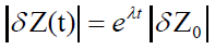 (8)
(8)
The maximal Lyapunov exponent is defined as:
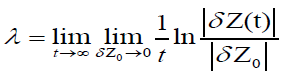 (9)
(9)
A Lyaponov exponent λ < 0 means that the system is stable at this point; if λ ≈ 1, it could be stable or unstable.
The Lyapunov exponent can often only be computed numerically. Most of the algorithms used to compute the Lyapunov exponent are based on a linearization of the system using an algebraic method (see [30] for example). As far as we know, no method exists that can be applied to a fuzzy model. We therefore applied the optimization routine from “NLOPT” to investigate the parameter space in terms of the maximal Lyapunov exponent. For example, two parameters p1 and p2 may be selected to study the Lyapunov exponent as the function of these parameters. Here, we decided to select P (related to the MMH) and f lux, which is known to strongly influence the systems behavior [21]. A map of the Lyapunov exponent was calculated for parameters P and f lux (Figure 9).

Figure 9: Map of the Lyapunov exponent; the larger the exponent, the darker (larger) the circles are.
Although the optimization routine cannot guarantee that the real maxi- mum will be found, there is evidence that λ < 0 for all sizes of the map
The transformation from a traditional system of ODEs to a dynamic fuzzy system can be applied in a straightforward manner. Experts/stakeholders are able to understand the system and to contribute their expert knowledge to the fuzzy models. This leads to easily understandable models, i.e. implementation follows a white box approach. The white box approach and expert participation enhance the credibility of the simulation. Experts are invited to add their own experience to model states that are outside the original rhs formulation of ODEs. One problem should be mentioned here. The model deals with scaled variables (often a range between [min, max] → [0, 1] is used). Scaling is pertinent because otherwise it is difficult to select the size of time steps, i.e. the number of iterations. Dealing with scaled variables helps modelers to learn the typical behavior of a dynamic fuzzy model for different applications. This is important because neither experts nor modelers are trained to build non- linear dynamic systems. Acceptance of scaling requiring a posterior descaling allows the number of variables in models to be reduced, making them simpler and more reliable. Descaling is required when results need to be compared with experimental findings. A dynamic fuzzy system should be analyzed using software that visualizes behavior under different settings of parameters. Monte Carlo simulations are an important tool in the ecological context, which is why simulation software should support this kind of analysis. Applying Monte Carlo simulation can deliver a distribution of possible states of a lake, for example, which can be used to establish a control strategy for protecting such lakes. It was shown that dynamic fuzzy models can produce a rich set of dynamics, including “Monod” kinetics. However, modelers do not need to know this kinetics in order to model the system. It suffices to describe dependencies in the form of rules over a set of membership functions. The example given shows how an expert/modeler applied his knowledge to describe the systems behavior. It is very important that the expert/modeler is not restricted by having to include such rules that are not part of the original DGL but belong to their practical experience. The effect is amazing, showing that experts/modelers already have the complicated behavior implicitly in their mind when developing fuzzy models
The stability of the dynamic fuzzy model was excellent, and was established without any need for fine tuning. Experts know which states of a real system are unstable, applying their supplementary experience to develop fuzzy models. n the traditional modeling process, modelers, often computer scientists, would only consult experts to a limited extent. This limited amount of communication often constitutes a problem, and can lead to suboptimal solutions. Another interesting problem connected to stability is the fact that dynamic fuzzy models can produce chaotic behavior [31]. In the approach discussed, fuzzy models are used to build a dynamic system, and not to control a system. We must still determine whether such a model can be chaotic. There is evidence against chaos in realistic problems due to expert knowledge, which is often more stabilizing [32].
The fuzzy simulator is now part of the spatial analysis and modeling tool SAMT, and can be used together with the SAMT core as a library inside Python programs. The high speed of dynamic fuzzy models enables them to be applied in spatially distributed environments. The dynamic fuzzy implementation is about ten times faster than a plant-water-soil model developed at ZALF [33], A dynamic fuzzy model can therefore be applied many times in a large region. It was possible to apply the dynamic fuzzy model introduced here to different parts of a lake to simulate a larger part or to the whole lake, for example. The main focus of this paper was to present a general method for handling nonlinear dynamic behavior based on fuzzy models. Even simple nonlinear dynamic systems can exhibit a rich and sometimes surprising behavior, including deterministic chaos. This rich behavior is necessary when seeking to model real systems. On the other hand, such simple models can be under- stood much more easily than complicated models. By reducing it to the main variables that describe a system, we have a great opportunity to understand the systems better, enabling us to move on from their relevant processes. A model is perfect when nothing can be removed.
This contribution was supported by the German Federal Ministry of Consumer Protection, Food and Agriculture, and the Ministry of Agriculture, Environmental Protection and Regional Planning of the Federal State of Brandenburg (Germany).