Research & Reviews: Journal of Pure and Applied Physics
ISSN: 2320-2459
ISSN: 2320-2459
Somayeh Nuri*
Department of Electrical Engineering, Urmia Branch, Islamic Azad University, Urmia, Iran
Received date: 27/12/2012 Revised date: 04/03/2013 Accepted date: 06/04/2013
Visit for more related articles at Research & Reviews: Journal of Pure and Applied Physics
The convergence behavior of the Least Squares Constant Modulus Algorithm in an adaptive beam forming application is examined. It is assumed that the desired signal and the interference are uncorrelated. The improvement in output SIR with each iteration of the algorithm is predicted for several different signal environments. Deterministic results are presented for an environment containing two complex sinusoids. Probabilistic results are presented for a constant modulus desired signal with a constant modulus interferer and with a Gaussian interferer. The asymptotic improvement in output SIR as the output SIR becomes high is also derived. The results of Monte Carlo simulations using sinusoidal, FM, and QPSK signals are included to support the derivations
CMA, Robust Algorithm, signal
The first CMA to be proposed was based on a Stochastic Gradient Descent (SGD) form [1]. The main drawback of this method is its slow convergence. A faster converging CMA similar in form to the Recursive Least Squares method is the orthogonal zed CMA [5]. Another fast converging CMA is the Least Squares CMA (LSCMA) [1,2,3,4], which is a block-update iterative algorithm. It is guaranteed to be stable and is easily implemented. Despite the generally accepted use of the LSCMA, few analytical results on its convergence have appeared in the open literature. The performance of the algorithm has instead been demonstrated through Monte Carlo simulation. The lack of analytical results is due to the difficulty of analyzing the non-linear CMA cost function. Existing work on the convergence behavior of CMA mostly deals with finding minima of the CMA cost function and finding undesirable stable equilibrium in equalization applications. A notable exception is the work by Treichler and Larimore on convergence of SGD CMA in an environment containing two complex sinusoids [6,7]. Their work predicts the output power of each sinusoid in a temporal filtering application. The Analytic CMA (ACMA) algorithm presented by van der Veen in [8] should also be noted. This algorithm solves directly for a set of beam former weight vectors that spatially separate a set of CM signals. The ACMA, although effective in many situations, is fairly complex and its behavior with closely spaced and/or low SNR signals is not clear. For these reasons it is recommended in [8] that the ACMA be used to initialize the LSCMA, and that several iterations of the LSCMA be used to find the optimal solutions for the weight vectors. In this paper we determine the convergence rate of the LSCMA in some simple environments, including: (1) high output SIR; (2) sinusoidal desired signal and sinusoidal interferer; (3) CM desired signal and CM interferer; (4) CM desired signal and Gaussian interferer. We assume that the interference is uncorrelated with the desired signal. The convergence rate is expressed in terms of the SIR improvement achieved with one iteration of the LSCMA. We first examine the situation where the LSCMA output SIR is high We show that if the interference is perfectly removable, each LSCMA iteration will increase the output SIR by approximately 6 dB. This result is valid for any CM desired signal (arbitrary angle modulation), and any uncorrelated interference. We next examine an environment containing two complex sinusoids, and show that the LSCMA output SIR can be predicted for each iteration.
The results are analogous to those presented in [8,9,10]. An environment containing two CM signals, each having random phase, is then considered. It is shown that the average behavior of the LSCMA in this environment is similar to the deterministic behavior in the two-sinusoid environment. Finally, an environment containing a CM desired signal and Gaussian interference is examined.
Analysis Frameworks
In this section we describe the general framework used to analyze the LSCMA. A key assumption is that the interference is uncorrelated with the desired signal. We essentially describe a simple way to measure the quality of the pseudo-training signal, d(n). If no background noise is present, the quality of the beamformer output y( n) will be identical to the quality of d(n). When background noise is present, the quality of y(n) is dependent on the quality of d( n) and the optimal output SINR. The optimal output SINR is in turn dependent on many factors, including the array geometry, the number of antennas, the number of incident signals, and the angle of arrival of each signal. The beamformer output signal at the kth iteration can be expressed, to within a multiplicative constant, as
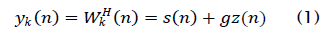
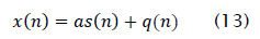
where s( n) is the constant modulus desired signal, z( n) is noise and interference, and the SINR of the beamformer output is controlled by g. Both the desired signal s(n) and the interference z( n) have unit variance. The hard-limiter output dk( n) will contain three components: (1) one component which is correlated with the desired signal; (2) one component which is correlated with the interference; and (3), one component which is correlated with neither the signal nor the interference. This last component is the result of intermodulation. Between the signal and the interference. We can express the hard-limiter output as
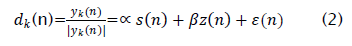
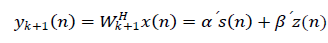
Where the scalars ∝ andβ control the desired signal power and the interference power, respectively, and ε(n) contains the intermodulation terms. We will now examine the relationship between the SINR in dk (n) and the SINR in the up-dated beam former output y(k+1). We initially assume that no background noise is present, and that the array has sufficient degrees of freedom to completely remove the interference. Given these assumptions, the optimal beam former output SINR is infinite. These assumptions are clearly not realistic, but this helps provide insight into the behavior of the LSCMA. As the block size N→∞, the updated weight vector wk+1 minimizes the MSE between yk+1(n) and dk(n),

We can express the updated beamformer output as
 (4)
(4)
Which, together with (12), allows the MSE to be written as

where we have made use of the fact that  are mutually uncorrelated. Clearly the MSE is minimized for
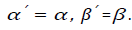 This implies that the signal component in the updated beamformer output will match the magnitude and phase of the signal component in the hard-limiter output. Thus the MSE between
![]() and the updated beamformer output
and the updated beamformer output is minimized when

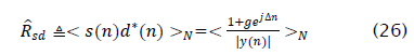
In order to find α and β, we calculate the cross-correlation of s(n) and z(n), respectively, with d(n). Note that
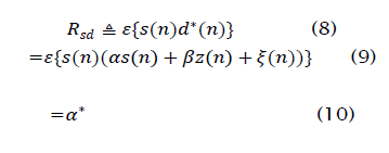
Similarly we have
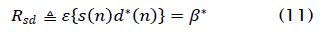
The SINR ρ in the hard-limiter output dk is
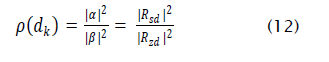
Since, we model s( n) and z( n) as having unit variance. Thus, the output SIR of the updated LSCMA weight vector can be determined from Rsd and Rzd. This requires that the probability density function (PDF) of the signal and the interference be known. To further illustrate the concepts behind this analysis framework, we will apply the LSCMA to a simple environment containing two uncorrelated complex sinusoids. The array configuration consists of two antennas, with the interelement spacing equal to λ/2, where λ is the carrier wavelength. One sinusoid, with a frequency of 5/1024, is incident from broadside to the array, which we define as 0°. This sinusoid is treated as the desired signal. The second sinusoid, with a frequency of -31/1024, is incident from 30°. This sinusoid is treated as the interfering signal. The amplitude of the first sinusoid is unity, and the amplitude of the second sinusoid is 0.9. The LSCMA is applied to this environment with the initial weight vector Wo = [ 1 0]. Thus the initial SIR is approximately -0.9 dB. The LSCMA block size N is set to 1024 samples. The periodogram of the initial beamformer output yo(n) is shown in Figure 1. The next step in the LSCMA is to hard-limit the beamformer output. The periodogram of the hard-limited beamformer output is shown in Note that the original sinusoidal frequencies are still present, along with intermodulation products. Also note that the relative amplitude of the desired sinusoid is now slightly higher relative to the interfering sinusoid. The exact change in relative amplitude is calculated later in Subsection 3.2. The next step in the LSCMA is to update the weight vector using the hard-limiter output in the same manner as a training signal. Figure 3 shows the periodogram of the updated beamformer output. As discussed earlier, the amplitude of each sinusoid in the updated beamformer output matches the amplitude of the corresponding sinusoids in the hard-limiter output. The intermodulation products are orthogonal to the signals present in the array data, and so have no effect on the weight update. It can be seen that the SIR in the updated beamformer output is approximately 3 dB higher than the initial SIR.

Figure 1: Periodogram of the initial beamformer output for the simple two-sinusoid environment. The initial SIR of 0.9 dB is indicated by the dotted horizontal lines.

Figure 2: Periodogram of the hard-limited beamformer output for the simple two-sinusoid environment. The SIR of 3.09 dB is indicated by the dotted horizontal line. Note that the calculation of SIR does not take into account the intermodulation terms.
We now derive an expression for the output SINR of the updated LSCMA weight vector when background noise is present. This will be shown to be dependent only on the optimal output SINR, the initial SINR, and the SINR gain provided by the hard limit non-linearity. The observed data is modeled as

Figure 3: Periodogram of the updated beamformer output for the simple two-sinusoid environment. The SIR of 3.09 dB is identical to the SIR in the hard-limiter outputs.
When background noise is present the interference and noise cannot be completely removed by beam forming. Independent thermal noise generated by each of the M receivers required for the M antennas in the array is a common source of background noise. The relationship between the SINR in dk(n) and the updated LSCMA output SINR is then somewhat more complicated.We now derive an expression for the output SINR of the updated LSCMA weight vector when background noise is present. This will be shown to be dependent only on the optimal output SINR, the initial SINR, and the SINR gain provided by the hard limit non-linearity. The observed data is modeled as
Where a is the spatial signature of the desired signal and q( n) contains the noise and interference. We assume that Rqq is
equal to the identity matrix. There is no loss of generality since whitening the data has no effect on the LSCMA. The crosscorrelation
vector Rxd is given by
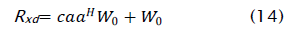
where W0 is the initial weight vector, and c is the square root of the SINR gain, with

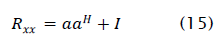
The covariance matrix of the data is
By the matrix inversion lemma
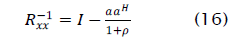
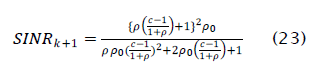
where p is the optimal output SINR . The updated weight vector Wk+1 is
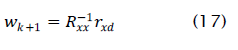
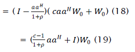
The output SINR of the updated weight vector is
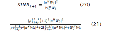
Since the initial SINR ρ0 is
the output SINR of the updated LSCMA weight vector can be written
We argued earlier that the output SINR of the updated LSCMA beamformer is equal to the SINR in the hard limited signal dk ( n) if no background noise is present. It is straightforward to show that
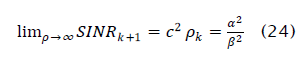
Which supports the argument made earlier. Also note that when c operation provides no gain, and
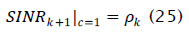
Here the output SINR of the updated weight vector equals the initial output SINR, as expected. In order for LSCMA to converge, the hard-limiter must emphasize the desired signal relative to the noise and interference. The effect of hard-limiting and other non-linear operations on communication signals and noise has been a topic of study since the 1950's, e.g., see [1,2,3,4,5] and references therein. A central motivation for this work is to understand the effect of non-linear amplifiers on communication signals, which are commonly used in satellite transponders. Non-linear processing has also been studied as a possible means for reducing the effects of noise and interference, e.g., [3,4]. These studies have clearly shown that hard-limiting and filtering a constant envelope signal will increase the SNR, even when the intermodulation components are considered. In fact, for a constant envelope signal, the hard-limiter becomes the optimal nonlinearity as the SNR tends to infinity [7-10].
Two Complex Sinusoid Environment
We now examine the behavior of the LSCMA in an environment where the antenna array receives two orthogonal complex sinusoids in the absence of background noise. We show that if the SIR at iteration k is known, the LSCMA output SIR can be predicted exactly for all later iterations. We also show that these results are a very good approximation with sinusoids having arbitrary, but well separated, frequencies. The results presented here are deterministic. Other results presented later examine the mean behavior of the LSCMA using a probabilistic framework. The beamformer output signal obtained with the existing LSCMA weight vector is modeled as
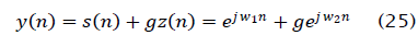
where  for integer ki. The parameter g determines the relative power of the sinusoids. In (43), s( n) and z( n) represent the desired signal and the interferer, respectively. The amplitude of the desired signal in y( n) is assumed to be unity, which has no effect on the behavior of the LSCMA. Temporal cross-correlation of the desired signal, s( n), and the hard-limiter output signal, d(n), is
Where  We note that since y is periodic
 ![]() is also periodic and may therefore be expressed as a Fourier series. The period
is also periodic and may therefore be expressed as a Fourier series. The period  of The function is real and even, so the Fourier series is given by
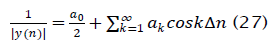
Where
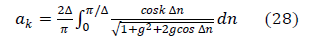
The Fourier coefficients given by (3.46) are independent ofΔ, which implies that the results to follow hold true for any frequencies W1 and W2, if these frequencies lead to orthogonal sinusoids. Substituting (45) into (44) yields
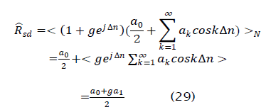
The Fourier coefficients a0 and a1 may be found using numerical integration. Using a similar approach for RZd yields The output SIR of the hard-limiter is
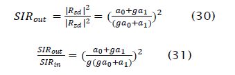
and the SIR gain is
Figure 4 shows the SIR gain (31) as a function of input SIR . Note that the SIR gain tends asymptotically to 6 dB as predicted by the high SIR analysis.
results presented in Figure 4 are now used to predict the output SIR of the LSCMA in an environment containing a sinusoidal desired signal and a sinusoidal interferer. A two element beamformer is simulated with the inter-element spacing equal to one-half the carrier wavelength, A. The desired signal is incident from broadside with an amplitude of one, and the interferer is incident from 30° off broadside with an amplitude of 0.9. The initial LSCMA weight vector is set to [1 0]T, so that the initial SIR ≅+0.9 dB. The block size is 1024 samples, with f1= 5/1024 and f2 = -31/1024. Table 1 compares the predicted results.

Figure 4: Improvement in SIR achieved by one iteration of LSCMA with sinusoidal desired signal and sinusoidal interferer.

Figure 5: Amplitude of both complex sinusoids in the beamformer output as a function of the number of LSCMA iterations. Solid line indicates predicted amplitude, '+' indicates amplitude measured in simulation.
measured output SIR at several iterations of the algorithm, which shows excellent agreement with theory. These same results are presented in an alternative manner in Figure 5. This figure shows the amplitude of each sinusoid as a function of the number of LSCMA iterations. A similar figure, showing the behavior of the SGD CMA in an environment with two sinusoids, appears in [10].

Table 1: Comparison of predicted and measured LSCMA output SIR in an environment containing two complex sinusoids.
We have examined the convergence behavior of the LSCMA in some simple environments. Algorithms such as Multi Target CMA, Multistage CMA, and Iterative Least Squares with Projection can be used for this purpose. The results presented here can form a basis for analysis of these multi-signal extraction techniques. Clearly the variance and distribution of output SINR obtained with the LSCMA is also an important area for investigation. We finally comment on the hard-limit non-linearity. For high SIR, the hard-limiter is the optimal non-linearity when the desired signal has a constant envelope. However, at low SIR other non-linearities can yield greater SIR gain. Thus it is possible that non-linear functions other than the hard-limit can be used to develop blind adaptive algorithms which converge faster for low initial SINR.